=TAKE(array, rows,[columns])
A description of each argument is listed here below:
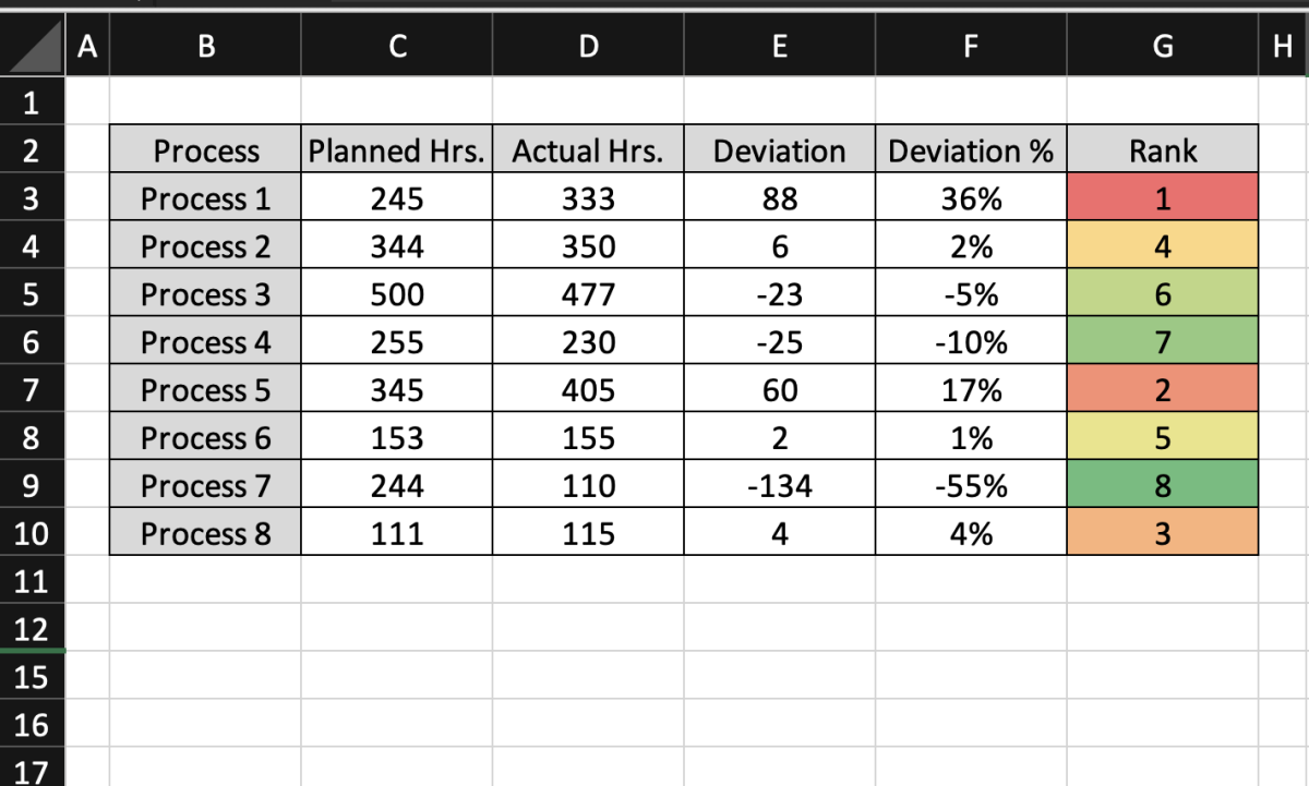
See how to use the TAKE function in the first example below where I duplicate a table and add formatting. In the next example, I cover displaying only the last rows and columns of a table.
In this example, I want to duplicate the whole table above and have it displayed in cell I2 to the right of the table. To start off I first type the being of the function formula.
=TAKE(
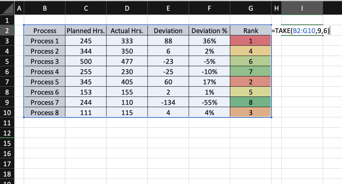
This is followed by selecting the range of cells to be duplicated followed by a comma.
=TAKE(B2:G10,
Next, the number of rows and columns must be indicated with a comma to separate these arguments. The formula is ended with a closing parenthesis.
=TAKE(B2:G10,9,6)
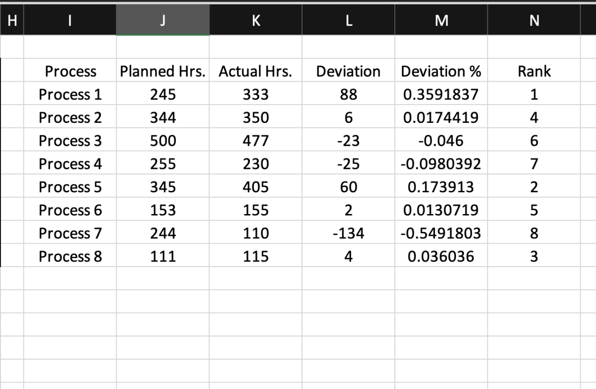
After the formula is entered, the data from the selected range will appear without formatting. Note that if you duplicate cells that don’t have data a zero will appear in those cells.
This data will change and update immediately when the parent table updates. What doesn’t update is the formatting of the duplicated table. The good news is that you can copy the formatting from the original table with the format painter.
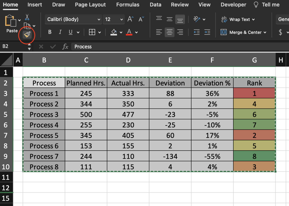
To copy the formatting from the original table select the table range of the original table and click on the format painter button.
Select the whole range of the duplicated table and the formatting will transfer.
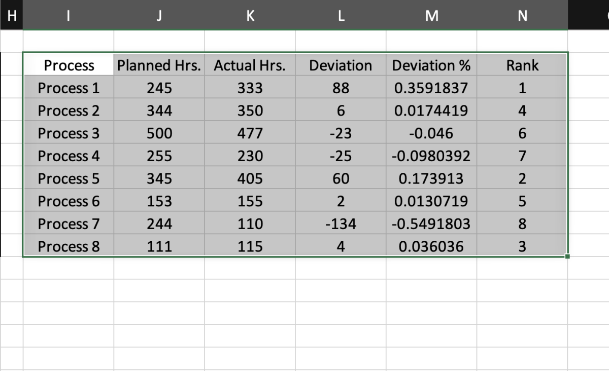
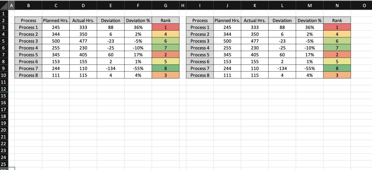
See the results below of the child table created by the take function and original table range.
While this example is a simplified case, the TAKE function can be used for a variety of reasons. Suppose that you have a report that is repeated throughout a workbook in multiple sheets. Instead of using macros or a large number of formulas to update the tables, it may be simpler to use the TAKE function to do the same task with one formula.
Take Data from the End of Columns and Rows
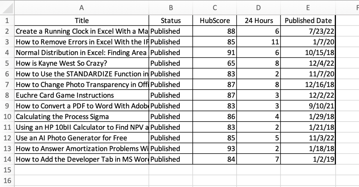
Negative numbers can play a part with the TAKE function to provide you with the last columns and last rows of data. Suppose have the data set below and only want to return data for the last tow row and last two columns.
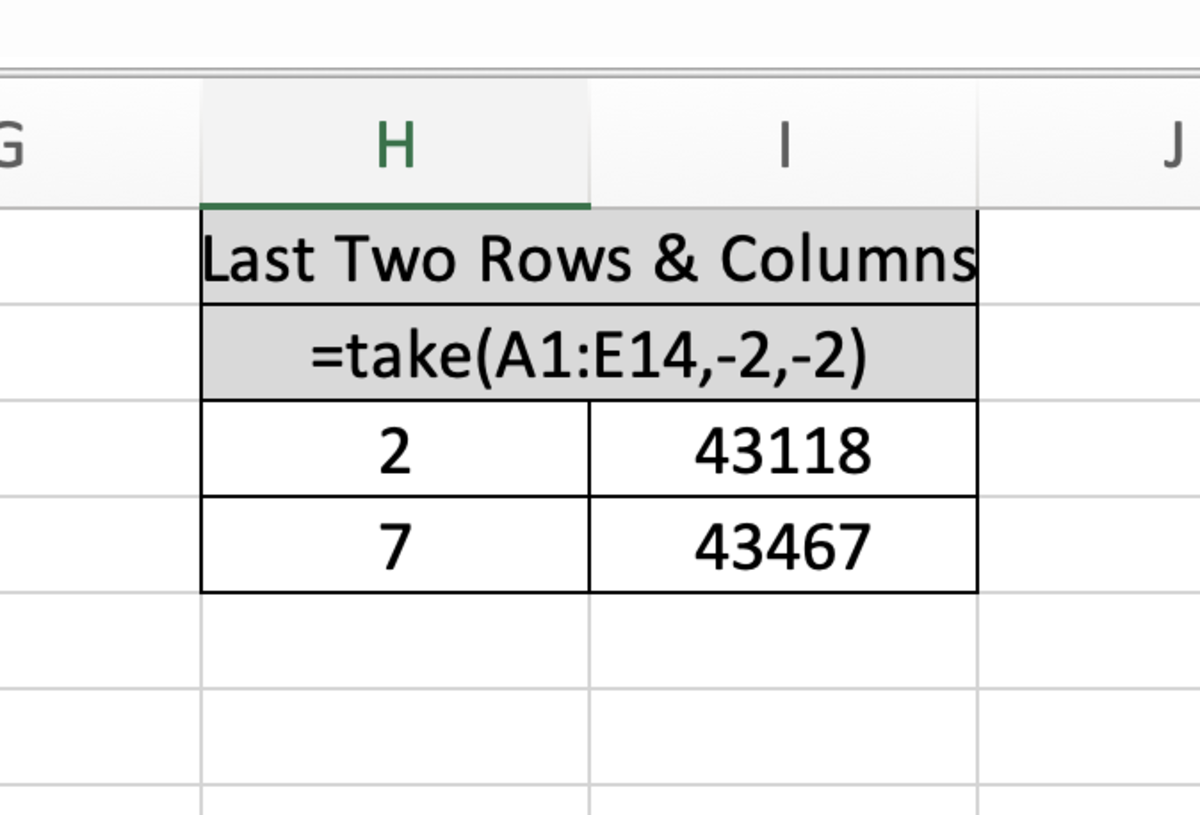
To accomplish this with the take function you would select the proper range followed by using a negative 2 for both the row and column arguments. Data from the last two rows and last 2 columns are displayed in the result below. The actual formula in the cell that contains the 2.
This content is accurate and true to the best of the author’s knowledge and is not meant to substitute for formal and individualized advice from a qualified professional.
© 2022 Joshua Crowder