Here’s a step-by-step tutorial with easy instructions to follow.
1. Determine Which Column You Would Like to Use to Calculate the Rank
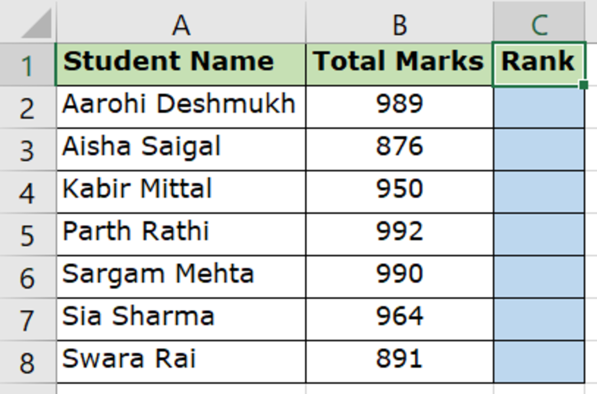
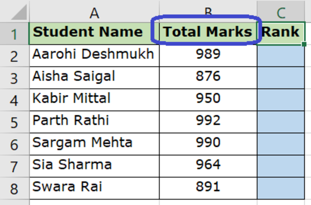
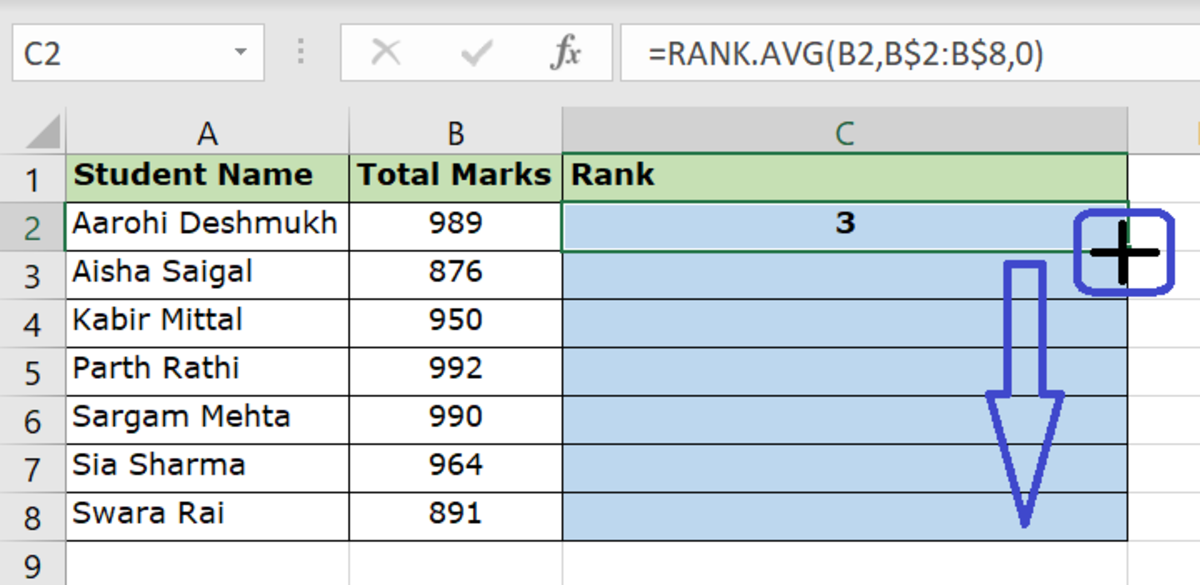
Let us assume we have a list of students and their total marks and we would like to rank the students based on their total marks. Here’s the sample data we are going to use to demonstrate how to do this. In our table here, we have a list of students and their total marks and we need to determine their ranks using the RANK capability within Microsoft Excel. So in this case, the column to be used to determine the RANK would be Column B, Total Marks of the students.
2. Use the Formula in the Cell Where the Rank Should Appear
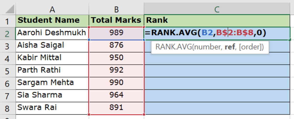
Formula to be entered in cell: C2 (That’s where the rank should appear) Formula to be used: RANK(number, ref, [order]) or RANK.AVG(number, ref, [order]) Keep in mind:
number stands for the cell where the number to be used to determine the rank exists. In this case number would be B2 because that cell holds the total marks. ref stands for the entire list of values that should be compared to determine the rank. In this case ref would be all values in column B that is B2 to B8). Do remember to add a $ symbol for this value so that the formula evaluates the entire table each time wherever this is copied. So B2:B8 becomes B$2:B$8. order stands for the order in which the values should be ranked. This can be either 0 (Descending Order) or 1 (Ascending Order) The difference between Rank and Rank.AVG is that you can use RANK.AVG to return the average rank if more than one number has the same rank. I am going to use RANK.AVG for our demonstration as our sample data anyway does not have same total marks for more than one student. So Rank and Rank.AVG will both give the same result.
3. Copy the Formula to the Remaining Cells
You could either copy and paste the formula in the remaining cells or you could drag the plus sign at the bottom right corner of the cell so that the formula gets copied to the remaining cells.
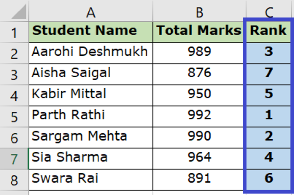
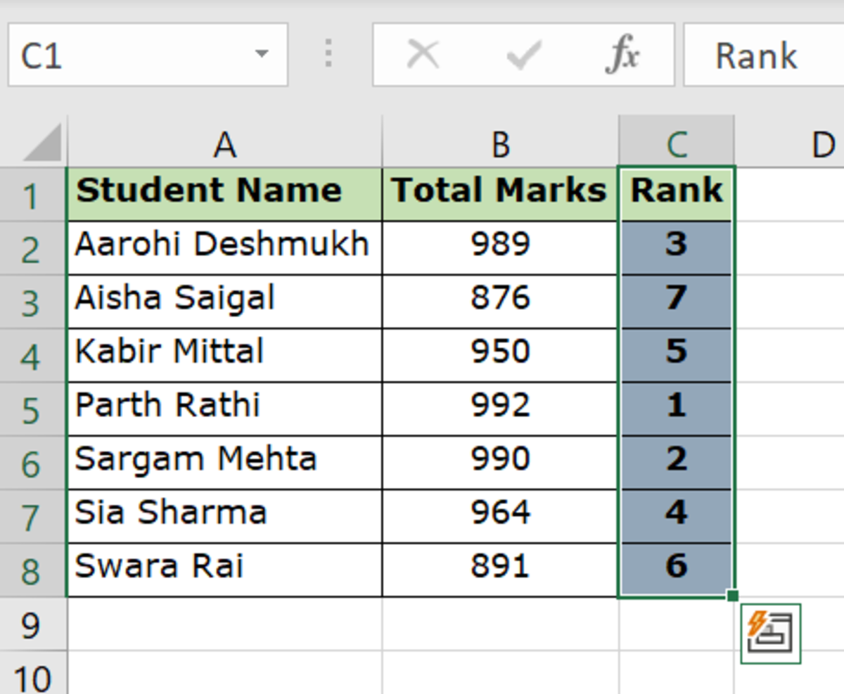
And Voila!
And done. Once the formula is copied to the other cells, it automatically ranks the entire list of students based on their total marks in this case. The result is the rank for each student has been calculated based on the total marks they have secured. This content is accurate and true to the best of the author’s knowledge and is not meant to substitute for formal and individualized advice from a qualified professional. © 2021 Petite Hubpages Fanatic
