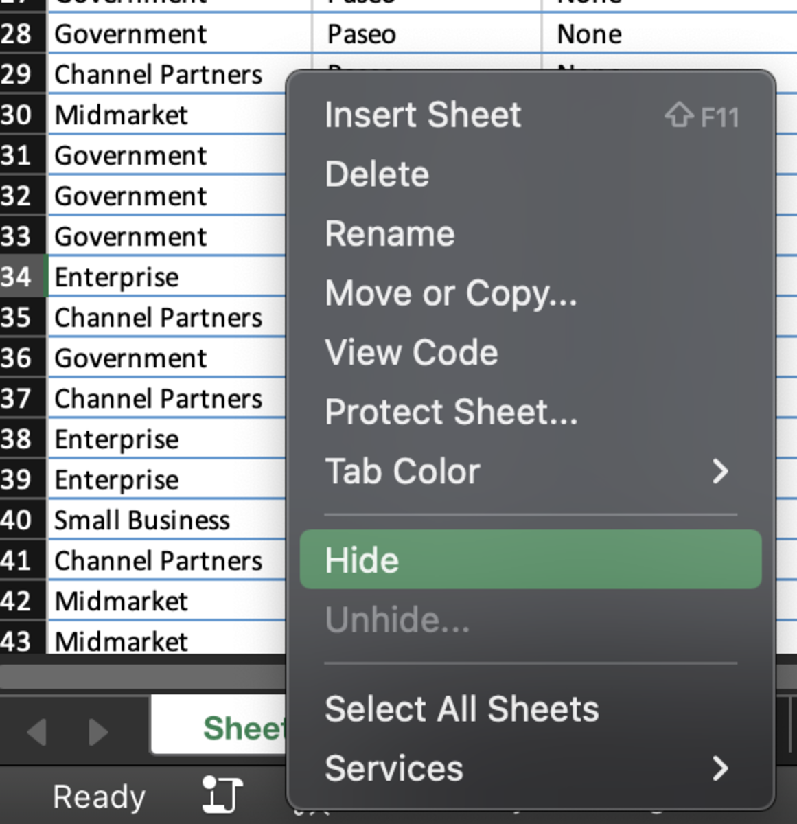
Hide Tabs
The are many instances where I don’t want the people that I’m working with to have access to some sheets in my workbooks. It is not a security concern and is more about keeping the integrity of formulas, references, and raw data. To hide tabs in Excel, simply right-click on the cell to be hidden followed by selecting the hide option. To bring the column back, right-click on any cell and select the unhide option. You can hide more than one tab so you will be given the choice of which tab to unhide if multiple are hidden.
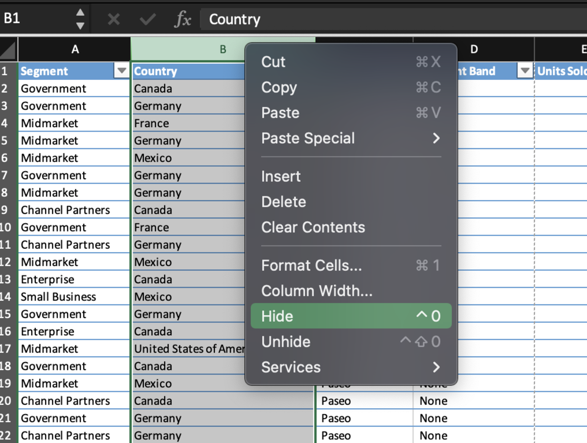
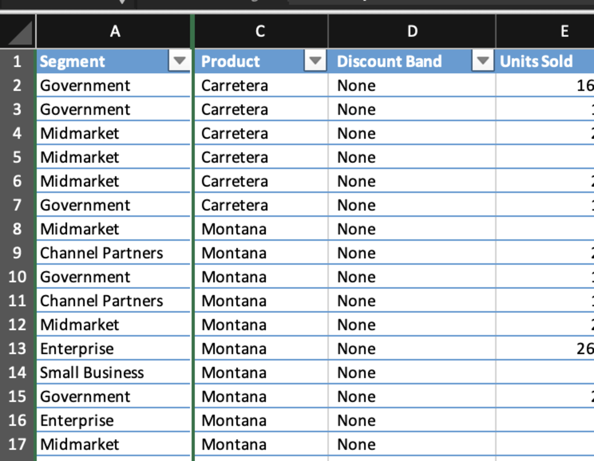
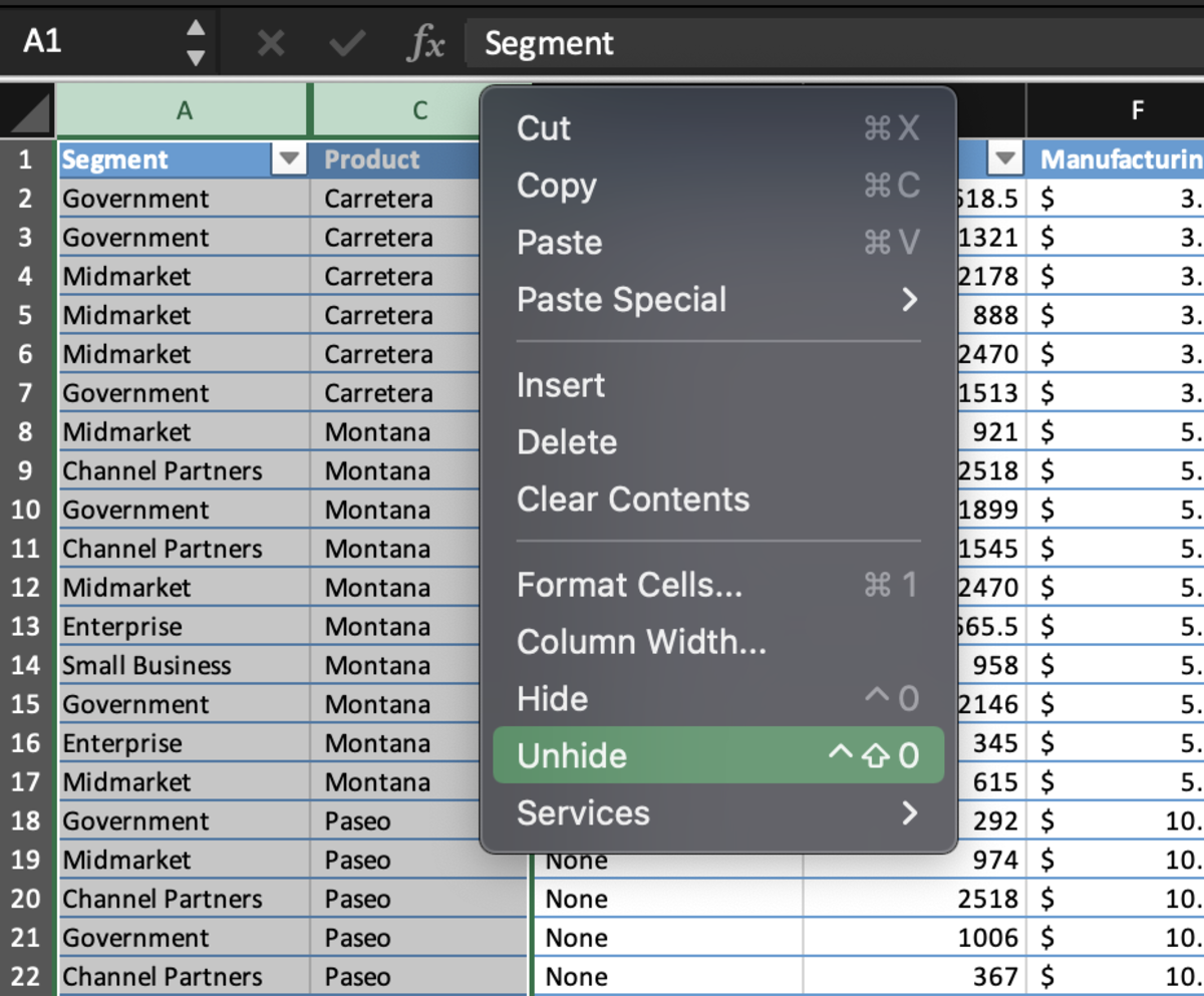
Hide Columns and Rows
Rows and columns can be hidden so you can protect certain attributes or records that appear in a table. To hide columns, select the columns to be hidden and right-click on the area. You will be able to tell where a column is hidden because you can see the gap in column letters. Notice that the B column was hidden and is now replaced by a gap in lettering. To bring the hidden column back, select the columns on both sides of the hidden column and right-click for options. Select the unhide option. It is also possible to hide multiple columns at once or separately. Rows are hidden in the same fashion as columns.
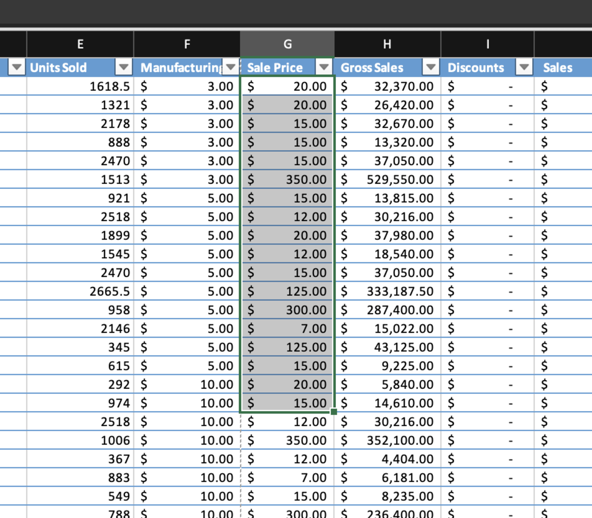
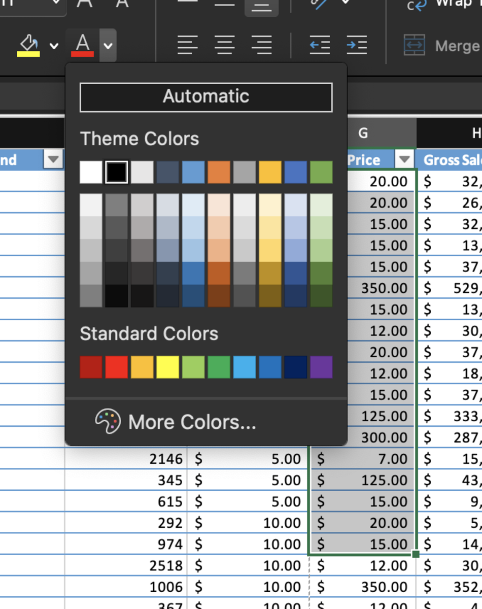
Hiding Text With Color
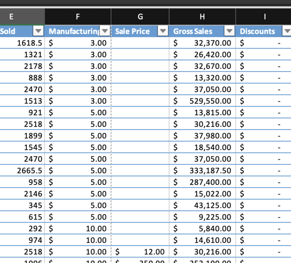
Changing the color of a text can be like hiding it in plain sight. First, select the cells that that value to be hidden appears in. Next, change the text color or the background color of the cell to hide the text with color. As you can see in the illustration below the text appears to be gone.
Hiding Formula Errors in Cells with Formatting
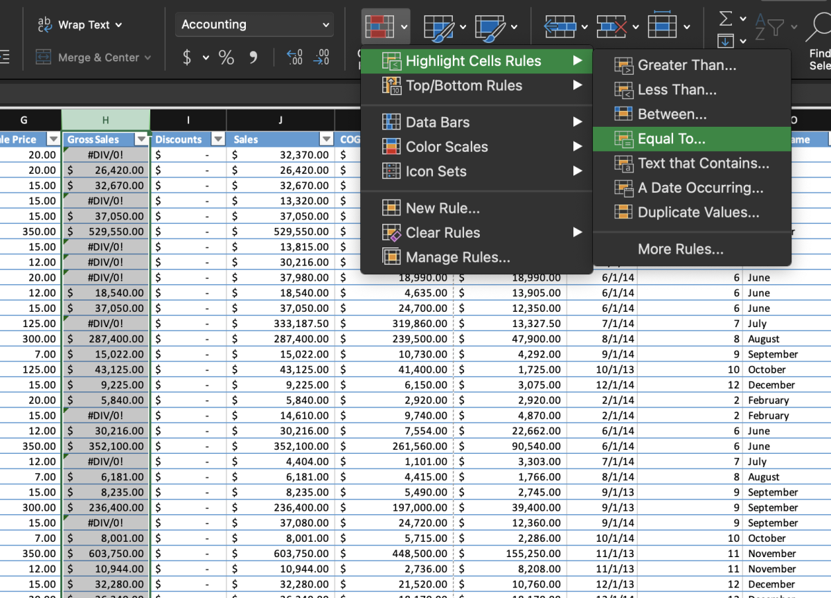
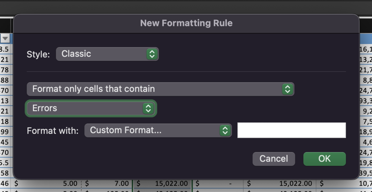
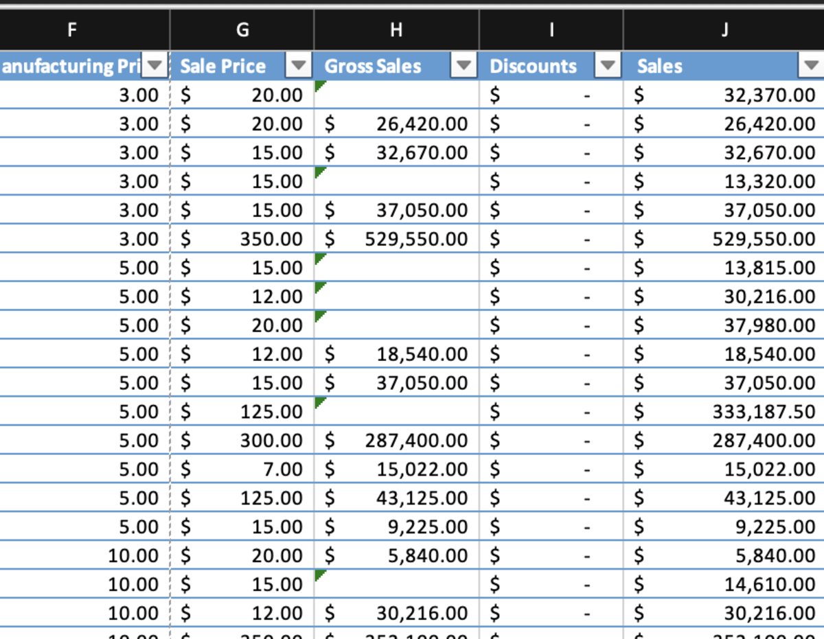
You can hide errors in cells on demand with conditional formatting that will only format a cell to hide the content of a cell if an error occurs. To hide your errors with conditional formatting start by selecting the data where the errors are likely to occur. Next, select the condition formatting button in the home tab of the ribbon. Select highlight cells rules and equals to for the options. Choose the errors option and change and select custom formatting. After the custom formatting is set for your situation (text was set to white in the example) any errors that occur will be hidden. The results are shown in the illustration below.
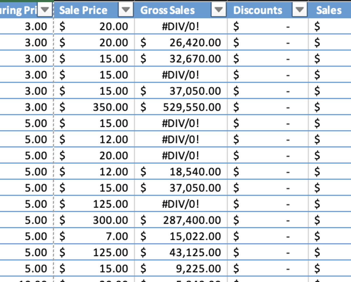
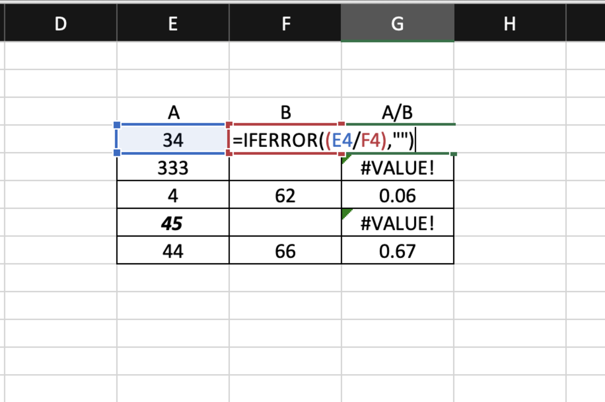
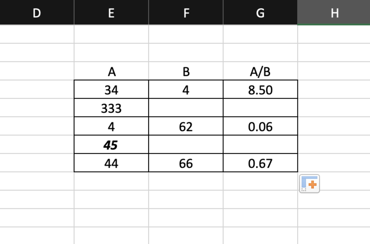
Hiding Formula Errors With the IFERROR Function
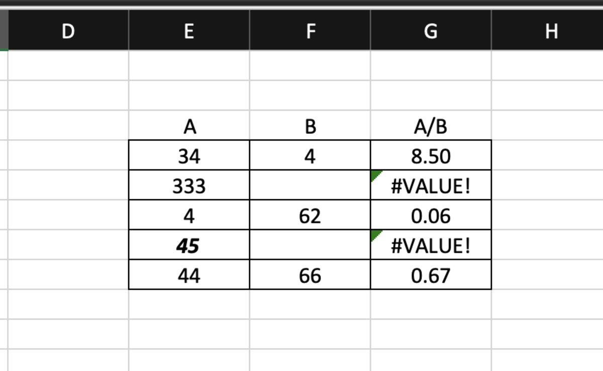
Sometimes hiding errors are more conveniently fixed through the formula that is causing the error to appear. Below errors are being caused because table column A of the table is being divided by zero is table column B does not have a cell value. The solution in this example is to use the IFERROR function in the existing division formula. The syntax of the IFERROR function can be seen below in bold. IFERROR(value, value_if_error) For the “value if error” section of the formula, I added two quotes together representing no space to keep the cell empty. After being applied to the first cell, the new formula is dragged down to the last calculation removing all errors. This content is accurate and true to the best of the author’s knowledge and is not meant to substitute for formal and individualized advice from a qualified professional. © 2022 Joshua Crowder