Pexels
Syntax of the IFERROR Function
The IFERROR function has a very simple syntax shown below. =IFERROR(value, value_if_error) There are two arguments that are required to use this function.
Value This needs to be a cell reference, a calculation, a function, or a series of functions. Value if Error Occurs This value can be what you want it to be. To display nothing simply use "" for this argument. For a space use " “. You may also add text or numbers without quotes.
Errors Messages That the IFERROR Function Can Hide
These references are provided to show what error messages the IFERROR function can hide. Each error is described in detail. Note that there may be more reasons for these errors to occur besides what is listed below. This needs to be a cell reference, a calculation, a function, or a series of functions. This value can be what you want it to be. To display nothing simply use "” for this argument. For a space use " “. You may also add text or numbers without quotes. #NULL! – Cell references are separated incorrectly. #N/A – Can’t find referenced data. #NUM! – Invalid numeric value. #REF! – Specific reference is not valid within an argument. #DIV/0! – Division by zero. #NAME? – Text within a formula is not recognized. #VALUE! – The wrong type of function or operand has been used.
IFERROR Example
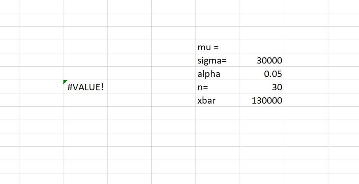
In the example below, I have an error because one piece of data is missing from one of my reference inputs for an equation. As a result, an error is displayed. Instead of having the error message “#VALUE1” appear when I have this error, I would like a custom message to appear for the user of the worksheet.
The IFERROR Solution
The formula that is causing the error is shown below. =2*(1-NORMSDIST(ABS((H12-H8)/(H9/SQRT(H11))))) The error is occurring because the cell reference H8 in the formula is missing from the H8 field. There are a few steps to replacing the error with a custom message.
Step 1. Click in the cell and position the cursor after the equals sign. Step 2. Type IFERROR( Step 3. After the last parenthesis, type a comma Step 4. Type the message that you choose to appear in quotes Step 5. End with a closing parenthesis and enter
Completing these steps will replace the error with a custom message.
Additional Resources
Below are two videos that will walk you through using the IFERROR function step-by-step if you are still having trouble.
IFERROR Demonstration
Remove DIV/0 Error Demonstration
This content is accurate and true to the best of the author’s knowledge and is not meant to substitute for formal and individualized advice from a qualified professional. © 2020 Joshua Crowder