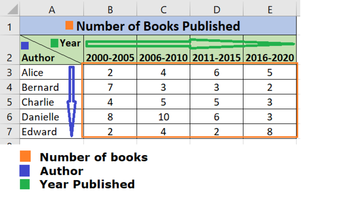
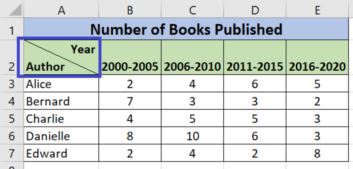
This technique comes in handy when you need to create complex table structures. Normally, when you need the cell in your Microsoft Excel Workbook to be split diagonally, you have two text values to be entered in that cell: one indicating the data in columns on the right, and the other indicating the data in the rows below. In our example today, let us assume the data we are using is a list of authors and the number of books published by them in different year ranges, where:
the data in numbers indicates the number of books published; the columns represent year ranges in chunks of five years each; and the rows represent the names of the authors.
We are going to use the diagonal cell splitting technique to represent the column and row headers for our sample data.
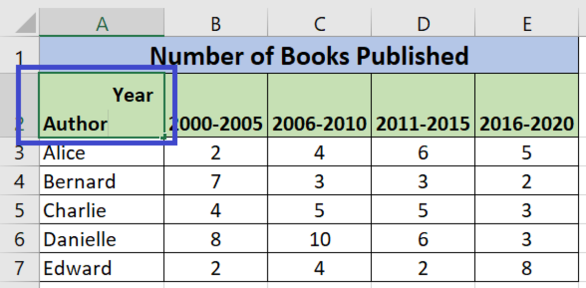
1. Type the Text in the Cell You Would Like to Split
The cell that needs to be split diagonally, holds two texts (per our example): Year and Author. Therefore, we need to type both Year and Author in the same cell. In our case the cell is A2. Our data cell is now ready to be split (with the data).
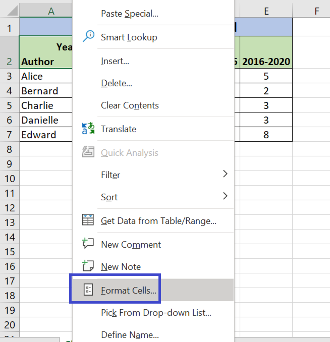
2. Format the Cell Using the Diagonal Border
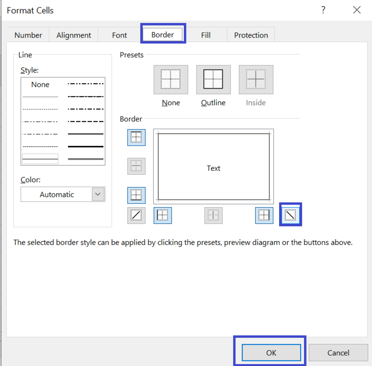
Right-click on the cell (A2) and select the option Format Cells. This opens up a new window with different options to format the selected cell. Go to the Border tab. Select the diagonal style border that resembles a black slash () and click ok.
And voila!
Done! The selected cell has been split into two halves diagonally. You have successfully learned how to split the cell diagonally like a pro! This content is accurate and true to the best of the author’s knowledge and is not meant to substitute for formal and individualized advice from a qualified professional. © 2021 Petite Hubpages Fanatic