A correlation coefficient (or the coefficient of correlation) can range in value from a negative to a positive where the sign indicates whether there is a positive or negative relationship between two sets of data. While the absolute value of this measurement shows the extent of an X and Y relationship, when squared (coefficient of determination), it shows the proportion of the variance of Y explained by knowledge of X and the reverse.
CORREL Function
The Purpose of the CORREL Function
Returning the correlation coefficient proves to be very useful when one needs to find the correlation between two arrays of data in a worksheet. This process can take seconds saving time on what are normally time-consuming calculations that are prone to human error.
Using the CORREL Function
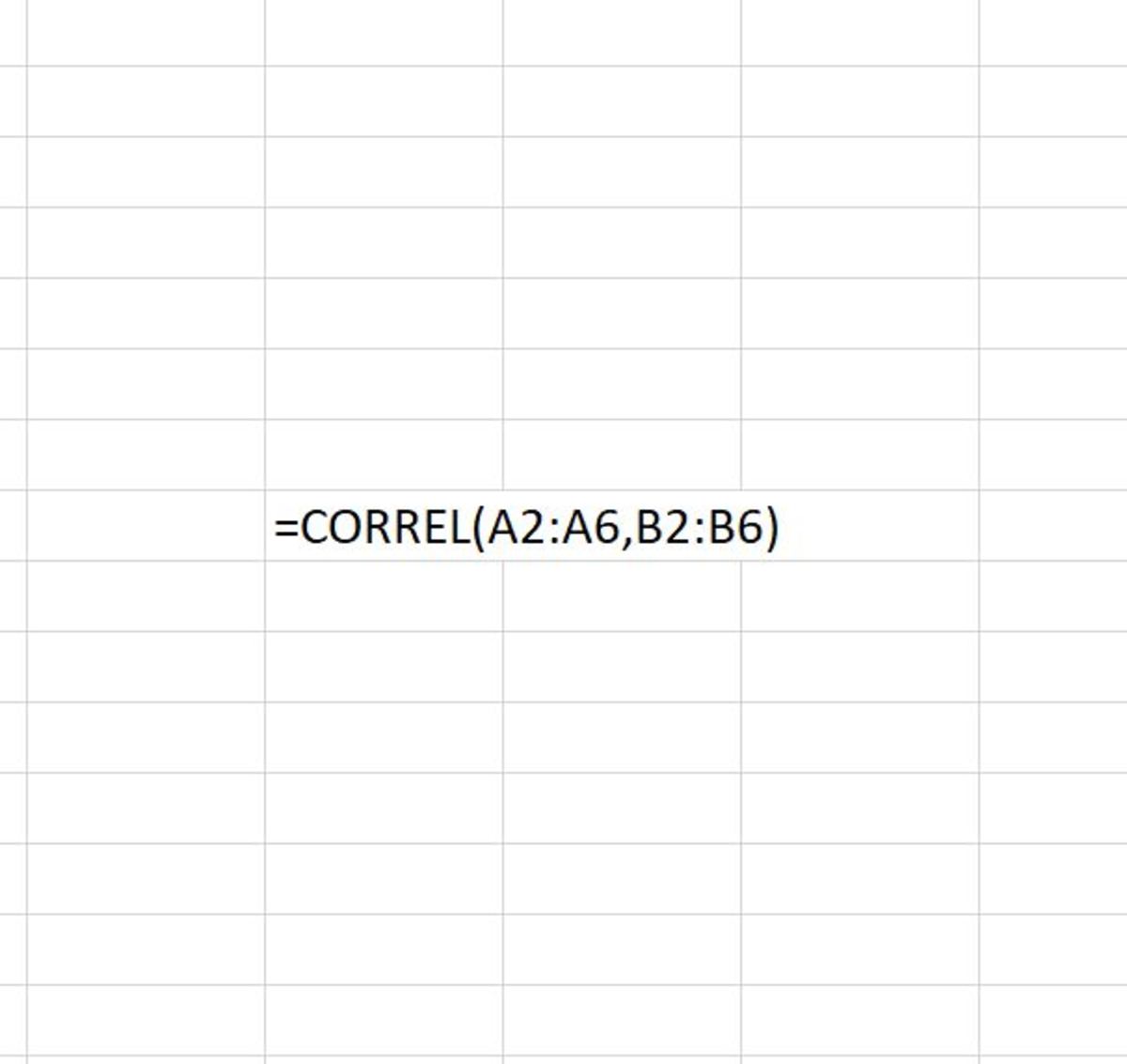
The CORREL function needs to be inputted in the form of a formula to work properly. To add this formula directly into a cell, a cell needs to be clicked in, and “=CORREL(” needs to be typed. Next, two arrays of data need to be selected. The syntax of the CORREL function can be seen here: =CORREL(array1, array2) These two arrays (array1 and array2) have to be the same size. By default, if a reference argument or array of data as text, an empty cell, or logical values, those cells will be ignored. The array data (numbers, range, named range, cell references) that are used to find the arithmetic mean must be entered and separated by a comma. This is then followed by closed parenthesis. After the formula is complete, the enter button can be pressed to return the correlation coefficient for the data.
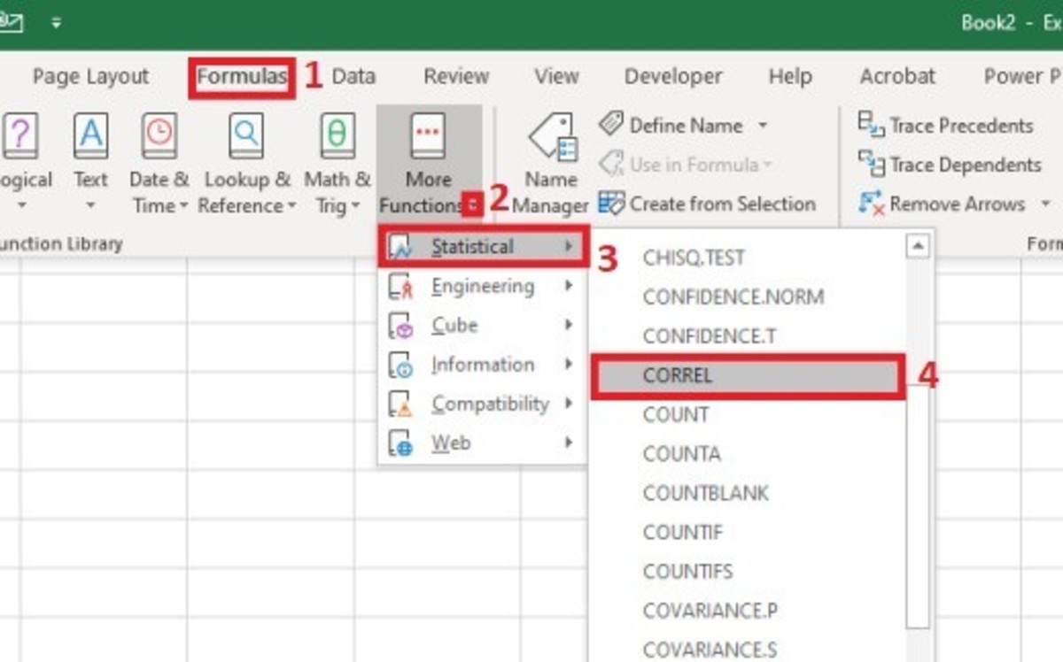
Inserting the CORREL FUNCTION
The CORREL function can be inserted into a cell with the assistance of a function insert tool. To use this tool, a cell must first be selected. Next, the formulas tab is selected and the “More Functions” button on the Excel ribbon needs to be clicked. The statistical selection from the list is chosen and the CORREL option needs to be clicked.
Selecting the CORREL Function From the Formula Tab
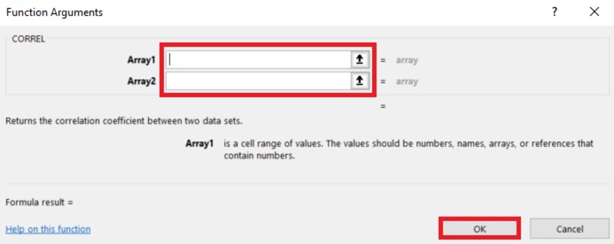
Next, the arrays of data can be added into the function arguments window by typing them in or by selecting the arrow buttons pointing up on the left side of the array fields. Notice the tips that appear under the array fields. After the arrays are added, the results also appear in the lower left-hand corner of this window. After each array is added, the okay button can be selected.
The Functional Arguments Window
CORREL Function Results
The CORREL function will return a positive number or a negative number. A number closer to positive 1 means that there is a strong positive relationship between the arrays of data. When the result is close to -1 there is a strong negative relationship between the arrays of data. When the result is close to zero there is not a close relationship between the arrays of data. There will never be a zero relationship because an error will result if this is the case. This content is accurate and true to the best of the author’s knowledge and is not meant to substitute for formal and individualized advice from a qualified professional. © 2020 Joshua Crowder