The LOOKUP Function Syntax
The LOOKUP function must be inputted like a formula to work. To manually add this formula to a cell the following steps need to be taken: Below the syntax of the LOOKUP function can be found in bold along with detailed explanations of each argument. LOOKUP(lookup_value, lookup_vector, [result_vector])
Lookup Value - This is a requirement. This is the value that the function searches for in the first vector (first column) unless the vector is specified. This value can be text, a number, a reference, or even a logical value. Lookup Vector - This is a requirement. This is a range that contains only one column if using the result vector or multiple columns is leaving the result vector out. These values can be numbers, text, or logical values. When used alone the first column of this range will be where the lookup value is trying to match and the last column will contain the corresponding result. Result Vector - This optional input is a range that contains only one column. A range that contains only one row or column. It is necessary for the result vector array to be the same size as the lookup vector. Note, if the result vector is not used that the lookup value or an error will display if the lookup value cannot be found.
LOOKUP Function Example
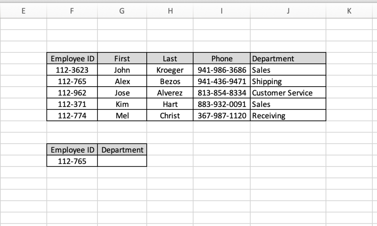
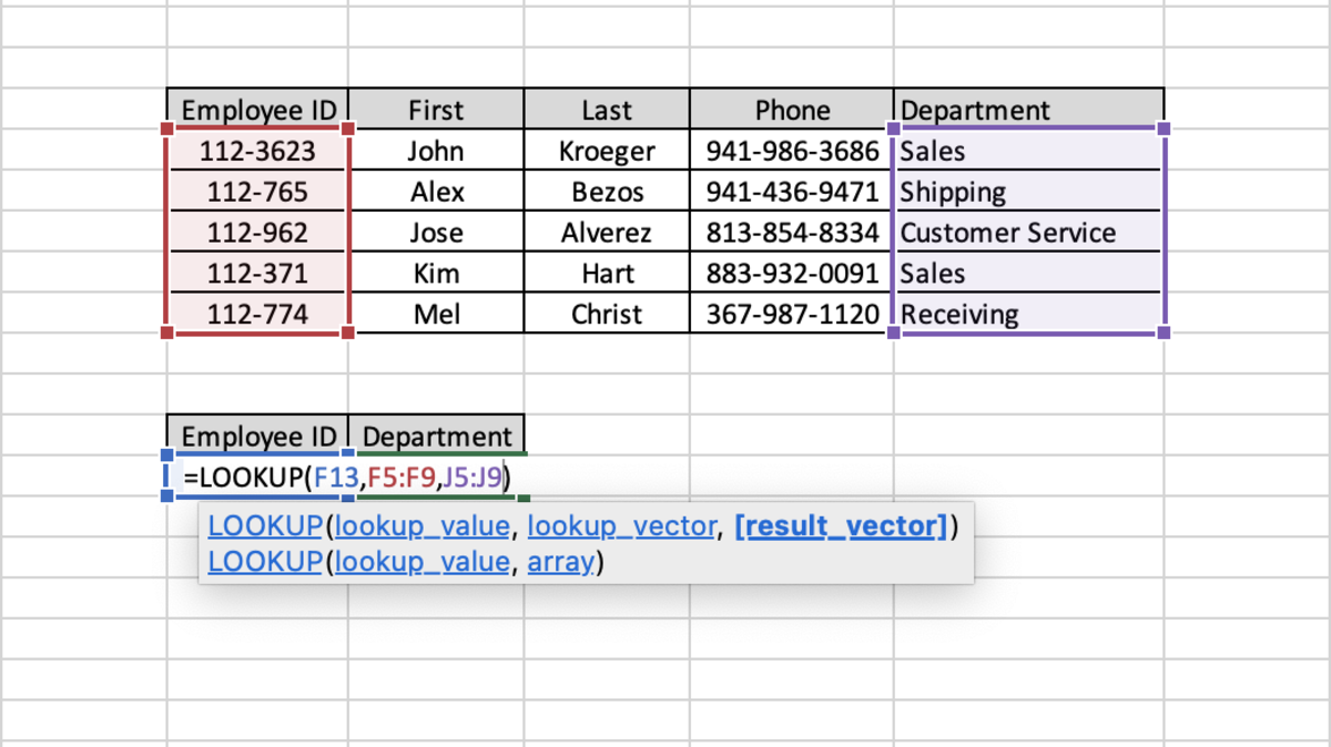
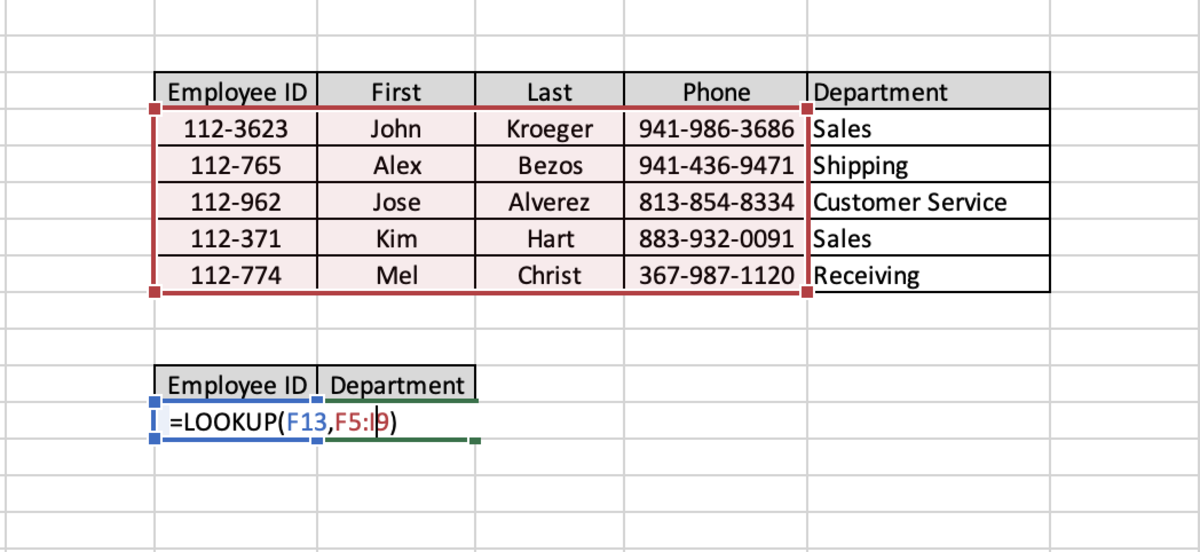
Suppose employee records in a worksheet need to be returned based on the employee’s identification number. This type of process can be made possible with the LOOKUP function. The spreadsheet below has employee data at a company and displays criteria about employees based on their employee ID. In the example below, the first option is used to return an item from the second array of departments. The employee ID number that appears in cell F13 will determine what department appears in cell G3 where the formula appears. In the second example below, only one array is used. In this situation, the value in the first column of the array will be looked up and the corresponding phone number data in the array will be returned because it is the last column of the array.
Inserting the LOOKUP Function
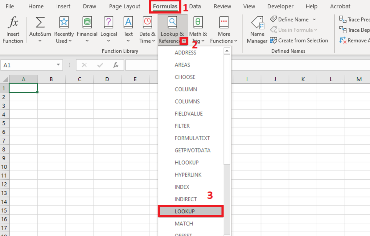
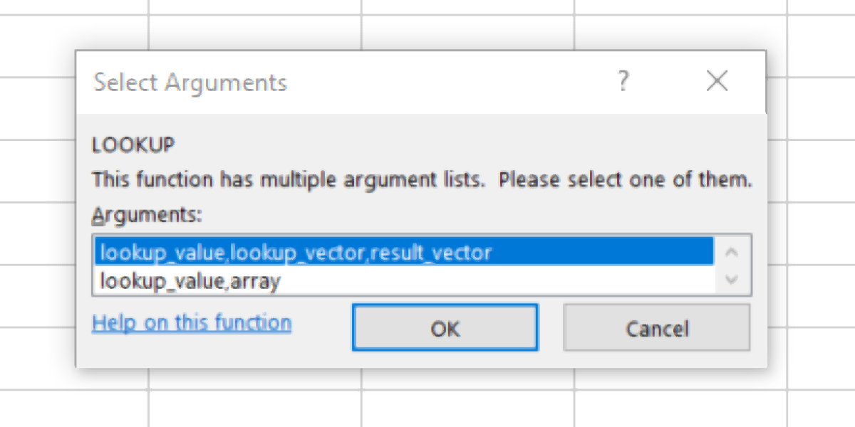
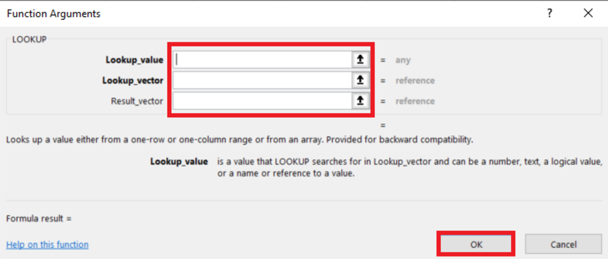
To insert this function from the function library a cell is first selected. Next, the formulas tab is selected and the “Lookup & Reference” button in the function library needs to be selected. A drop-down will appear and “LOOKUP” from the list should be chosen. Next, you will need to select one of two argument configurations that you would like to use. Below I choose the vector option and the fields are ready to input data. The insert option is great because when you clicked in the argument fields instruction are given to help you enter the function. Additionally, the result will be displayed before you enter the function by selecting OK. This content is accurate and true to the best of the author’s knowledge and is not meant to substitute for formal and individualized advice from a qualified professional. © 2022 Joshua Crowder