Using the RAND Function in Excel
The RAND function should be typed as a formula for it to operate. To manually add the RAND function to a cell, a cell needs to be clicked before “=RAND()” is typed. Once this formula is completed, it will create a random number after being entered into a cell. The RAND function will return a random number under 1. You may end up with a lengthy number under 1 if you don’t format the cell you are using with the appropriate place value. To obtain a whole number simply multiply the RAND function by 100 and set the place value to round up to a whole number. Each time this function is used a random number between 0 and 100 will be retrieved.
Inserting the RAND Function in Excel
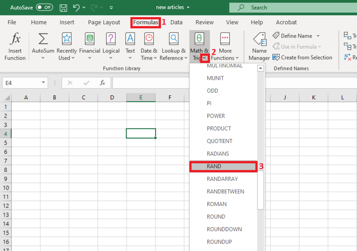
The Rand function can be inserted into a cell with the Excel insert function tool. This method may be used if one forgets the syntax of the function. To begin using this method a cell is selected. Then, the formulas tab is selected and the “More Functions” button on the Excel ribbon is selected. The statistical selection from the list is then chosen. A drop-down will appear, and the RAND selection will need to be chosen.
Selecting the Rand Function From Formulas
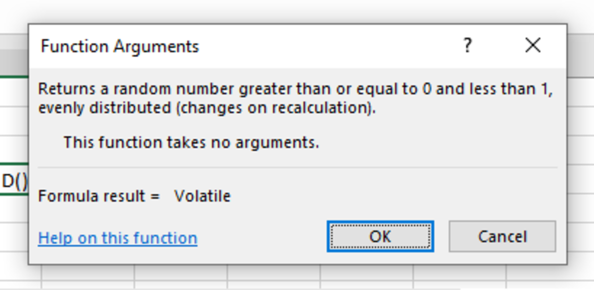
Next, a window will appear that wants you to acknowledge that this function does not require an argument. Click the OK button and the random number will display. After the “function arguments” window appears, a cell reference can either be typed in or selected from the worksheet by clicking on the up arrow to the right of the value field. Notice the reference under the value field. This reference indicates what value will be returned depending on what type of data is referenced. Once the reference is entered into the value field a preview of the number that will be displayed will appear in the bottom left-hand corner of this window. Additionally, any data can be entered into the values field to see what type of data it is. After the reference is selected, click on the OK button.
Create a Random Number Button in Excel
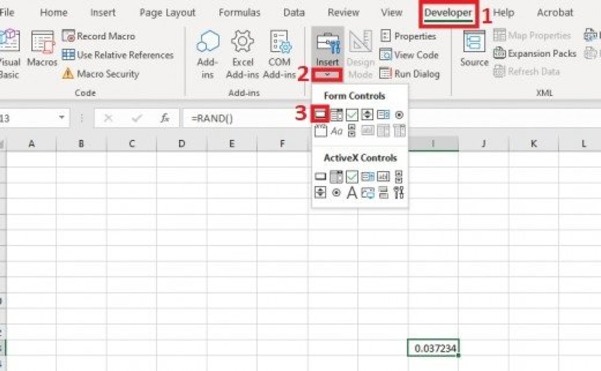
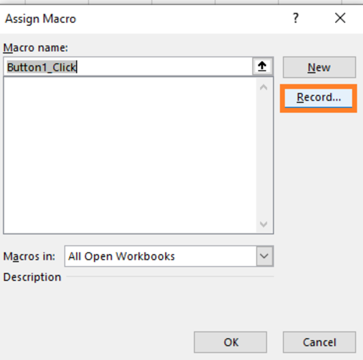
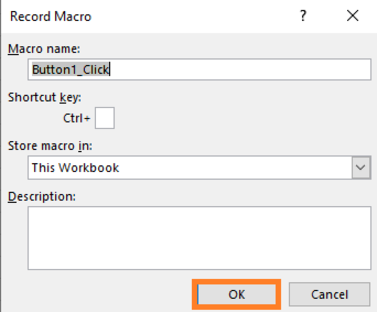
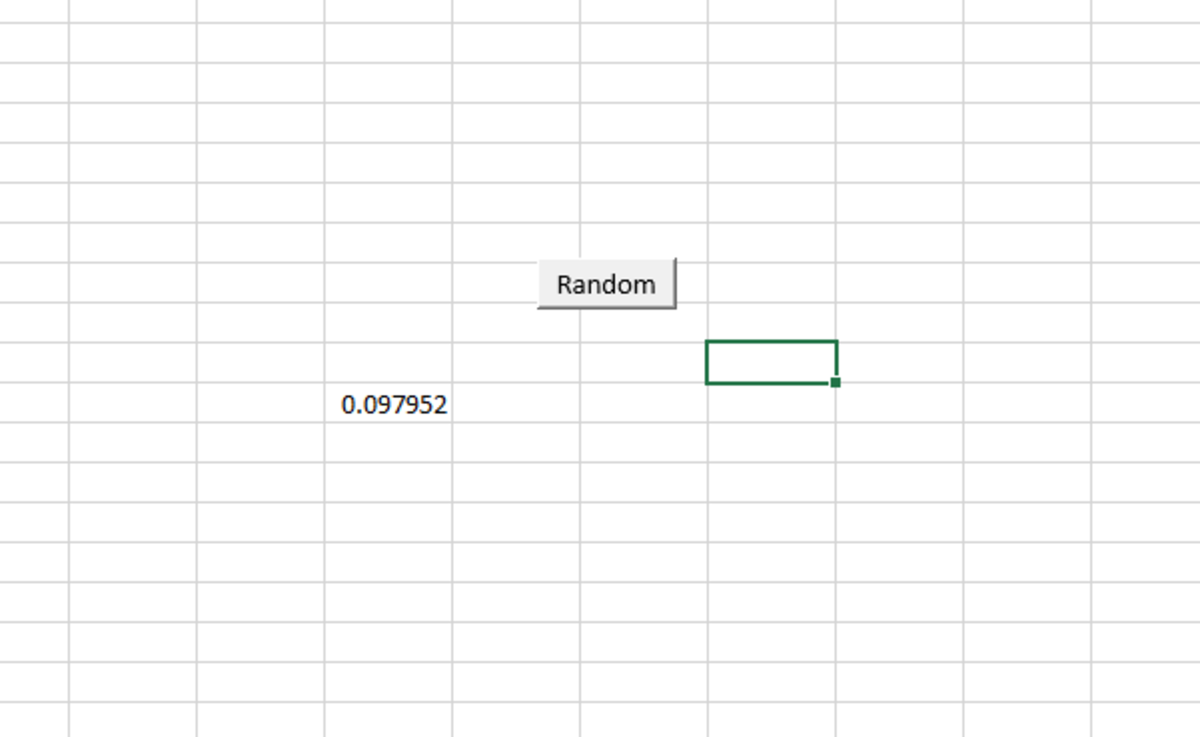
Here I explain step-by-step how to easily create a button that will cause the RAND function to refresh. To get the rand function to refresh without going through this trouble simply press the F9 key. Creating a button in the worksheet to do this only requires a few steps. To follow along you will need to enable the developer tab in Excel. If you don’t have this tab enabled, learn how here. Start by adding the RAND function to a cell. Next, click on the developer tab, select the insert button, and select the command button icon in the top left-hand corner of the form controls section. With the cursor, draw a square or rectangle while holding down the left mouse button. When the assign macro window appears, click on the record button. After the record button window appears, click the OK button. Press the F9 key once and then click on the little square in the bottom right-hand corner of your screen. By following these steps, you essentially record yourself pressing the F9 key and assigning that function to the button. To edit the name of the button, right-click on it followed by a left-click on the text to edit it. Each time a random number between zero and one is needed the button can be pressed.
Rand Function Button
This content is accurate and true to the best of the author’s knowledge and is not meant to substitute for formal and individualized advice from a qualified professional. © 2020 Joshua Crowder