How to Use the STOCKHISTORY Function
This function has four different arguments that determine how stock data will be displayed. Each argument is listed below: The full syntax of this function is shown below: Yes, this can be typed out but I show you how to insert this function in the next section. This method decreases the risk of error in functions that require multiple criteria.
Inserting the STOCKHISTORY Function
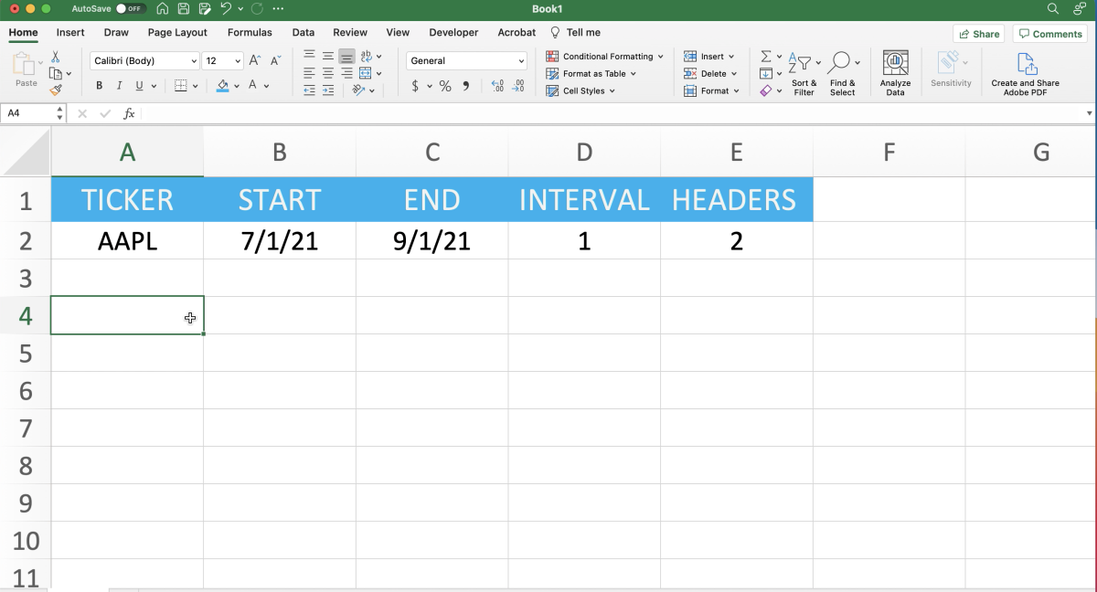
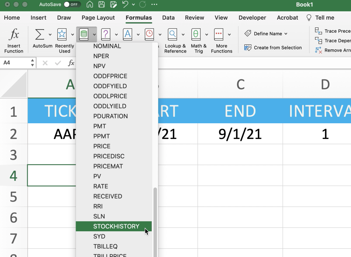
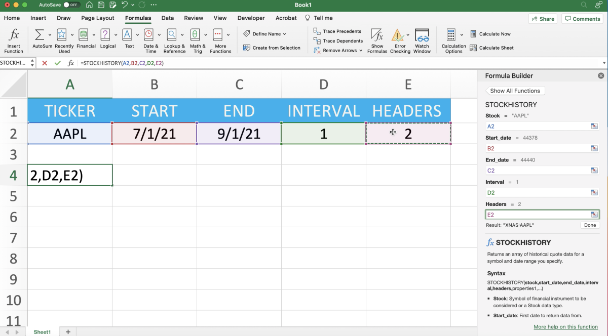
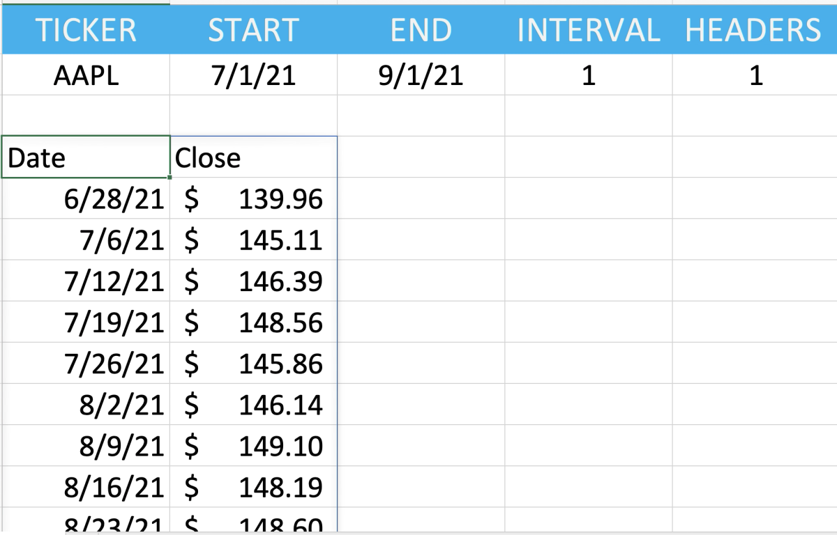
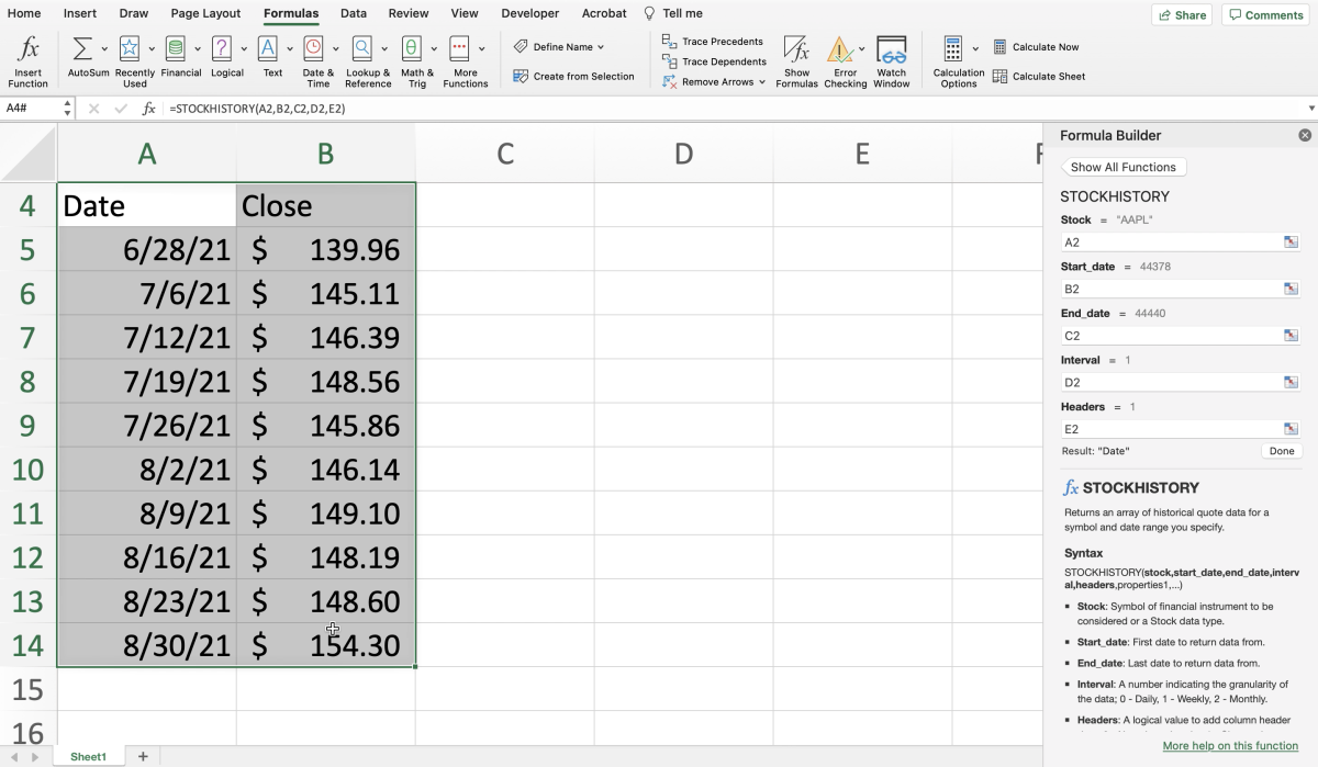
The best way that I found to use this function is to have the data laid out in such a way as to avoid errors. This was completed in the illustration below with headers to describe the data. Start the process of inserting the function by clicking into the cell where you want the top left-hand corner of your data to appear. Note that the more criteria that you select, the more columns will populate to the right of this area. The number of rows that populate is dependent on the date range and interval. Next, the formulas tab can be chosen, and the drop-down labeled financials can be clicked on. Select STOCKHISTORY from the list of financial functions. The formula builder should appear on the right side of the screen. Click in each of the blanks one at a time, and select the references related to the arguments that they represent. After all the blanks are filled, select the done button.
Avoid the Spill Error
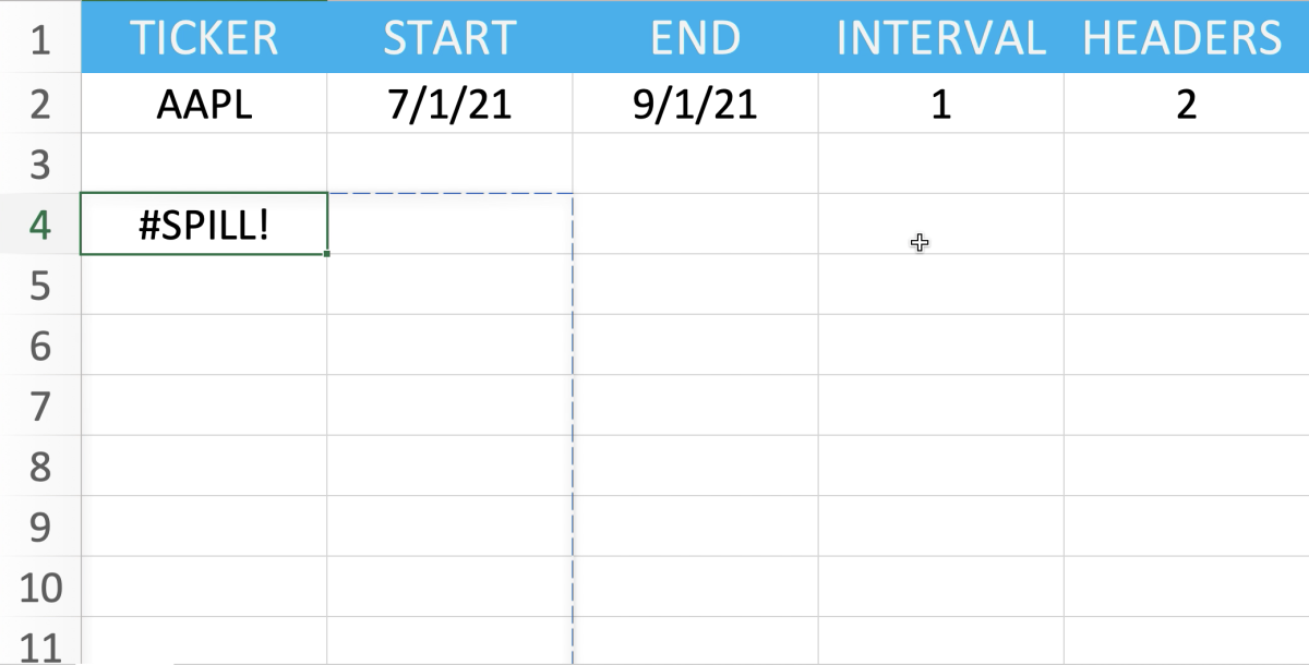
A common error that occurs with these kinds of functions is a spill error. This may occur if you used this function more than once in the same area of cells. To remedy the error, delete all the rows where the last function displayed data and try again. Another option would be to add the function to another cell. The data should appear below and to the right of the cell where the formula was added (as long as you are connected to the internet). You should be able to change the criteria in the referenced cells to manipulate the outcome of the function.
Adding a Graph
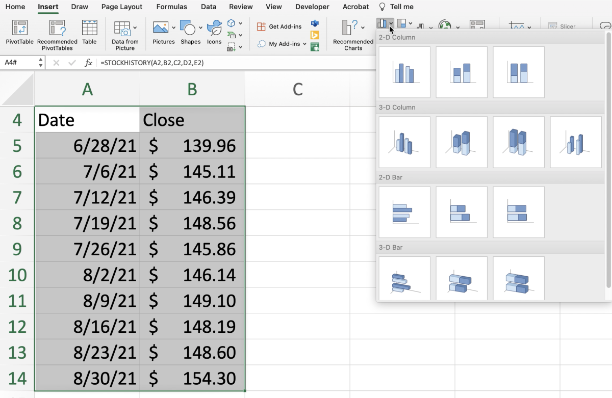
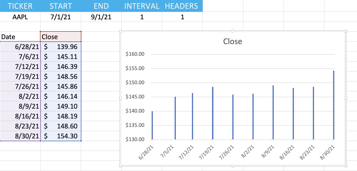
One option that can be used to give you a better visual of your data is to insert a graph. Excel has a wide variety of graphs and can add value by showing trends in the data providing you with a quicker way to analyze a large data set. To add a graph, start by selecting each column of data. Next, select the insert tab and choose a line graph or bar graph from the area that contains the graph icons with drop-down menus. After a graph has been selected, you may want to drag the corners of the graph to resize it to fit the spreadsheet. This content is accurate and true to the best of the author’s knowledge and is not meant to substitute for formal and individualized advice from a qualified professional. © 2022 Joshua Crowder