The least squared method is used in regression analysis to find the line that best fits. So, this method draws a line to show the relationship between points for a given data set.
How the TREND Function Works
The TREND function must be inputted into a cell like a formula. To enter the TREND function into a cell, follow these steps with details about each variable:
Set the constant to TRUE to calculate y = mx + b normally. Omit a setting to calculate y = mx + b normally. Set the constant to FALSE so that b is equal to zero. In this case, the m values will be adjusted so y = mx.
The syntax of the TREND function is shown in its entirety below: =TREND(known_y’s, [known_x’s], [new_x’s], [const])
Inserting the Trend Function in Excel
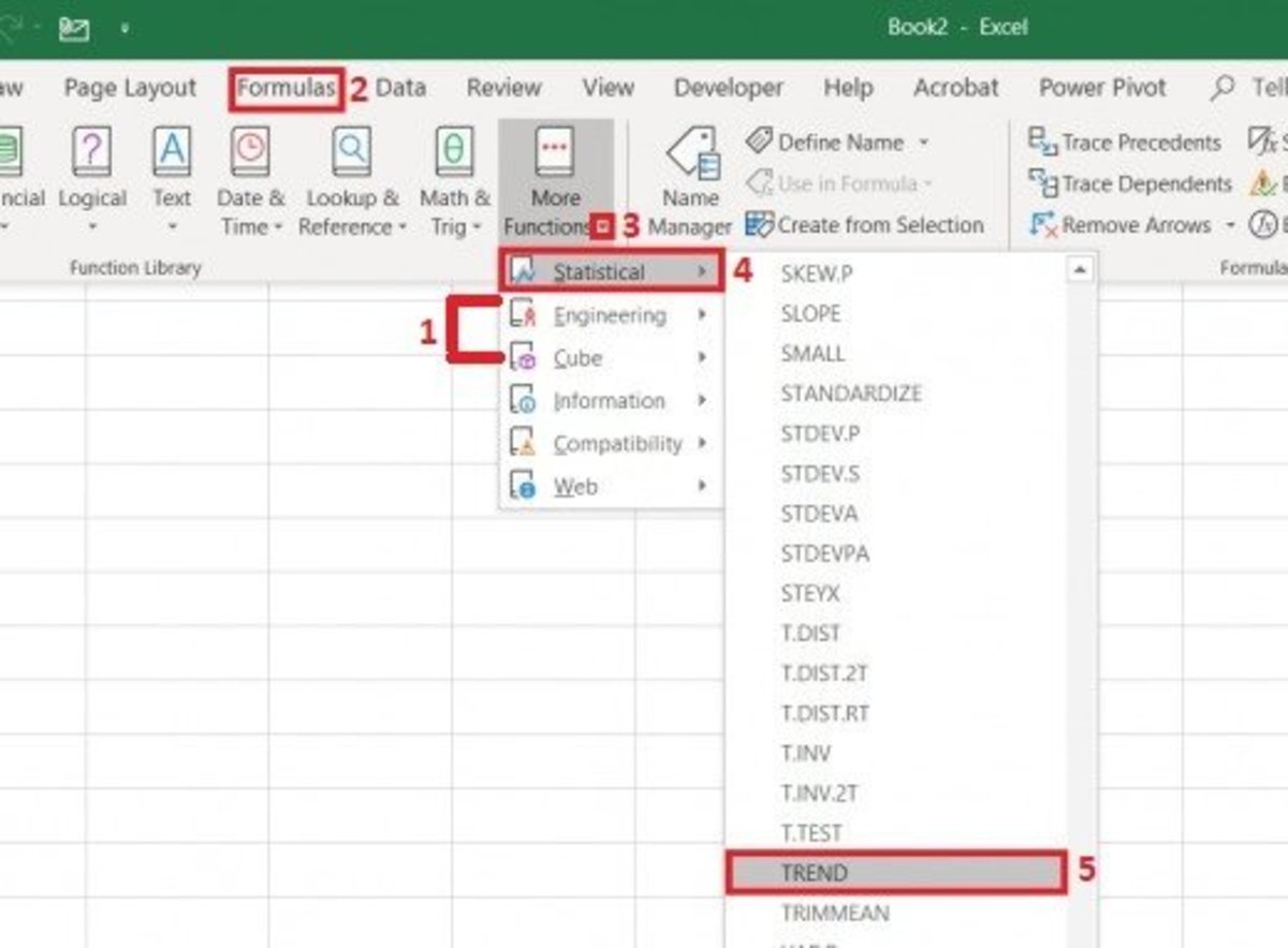
The TREND function can be added by inserting it into a cell from the statistical functions list. By using this method, Excel will walk you through the creation of the function by allowing you to enter function variables into fields with explanations for every variable entry. This method is good for this type of function since multiple variables are used and could get mixed up while creating the formula manually by typing it in a cell. To use this insert type method: Each step in this process is shown in the illustration below.
Selecting the Trend Function
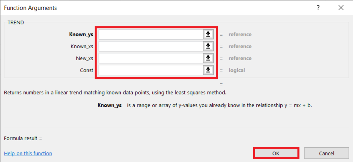
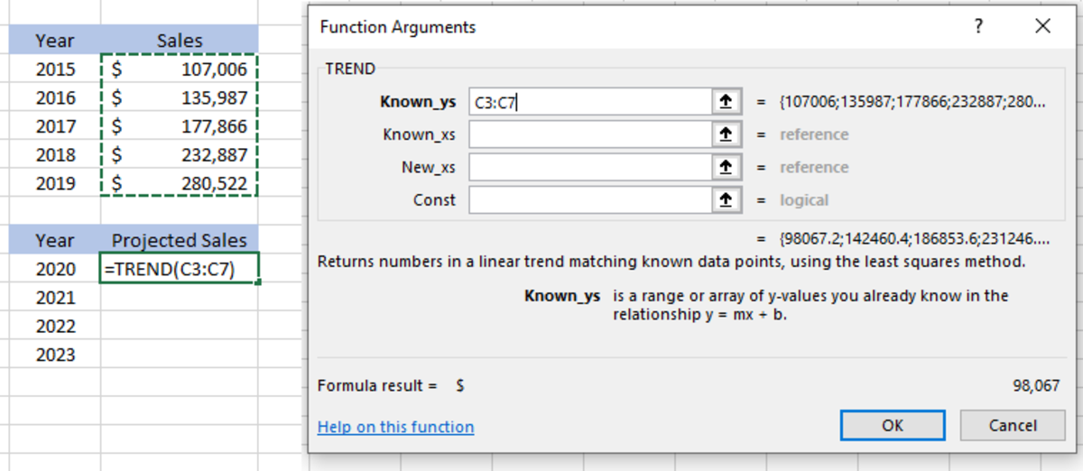
Next, a functions argument window appears where each of the function’s variables can be added. The arrays can either be typed in or selected from the spreadsheet by clicking on the arrow to the right of the array fields. The constant value (TRUE or FALSE) can be typed or a cell reference containing a value can be chosen by clicking on the arrow to the right of that field. Remember that the constant value is optional and not needed for general trend forecasting. Click the OK button when finished.
Functional Arguments Window
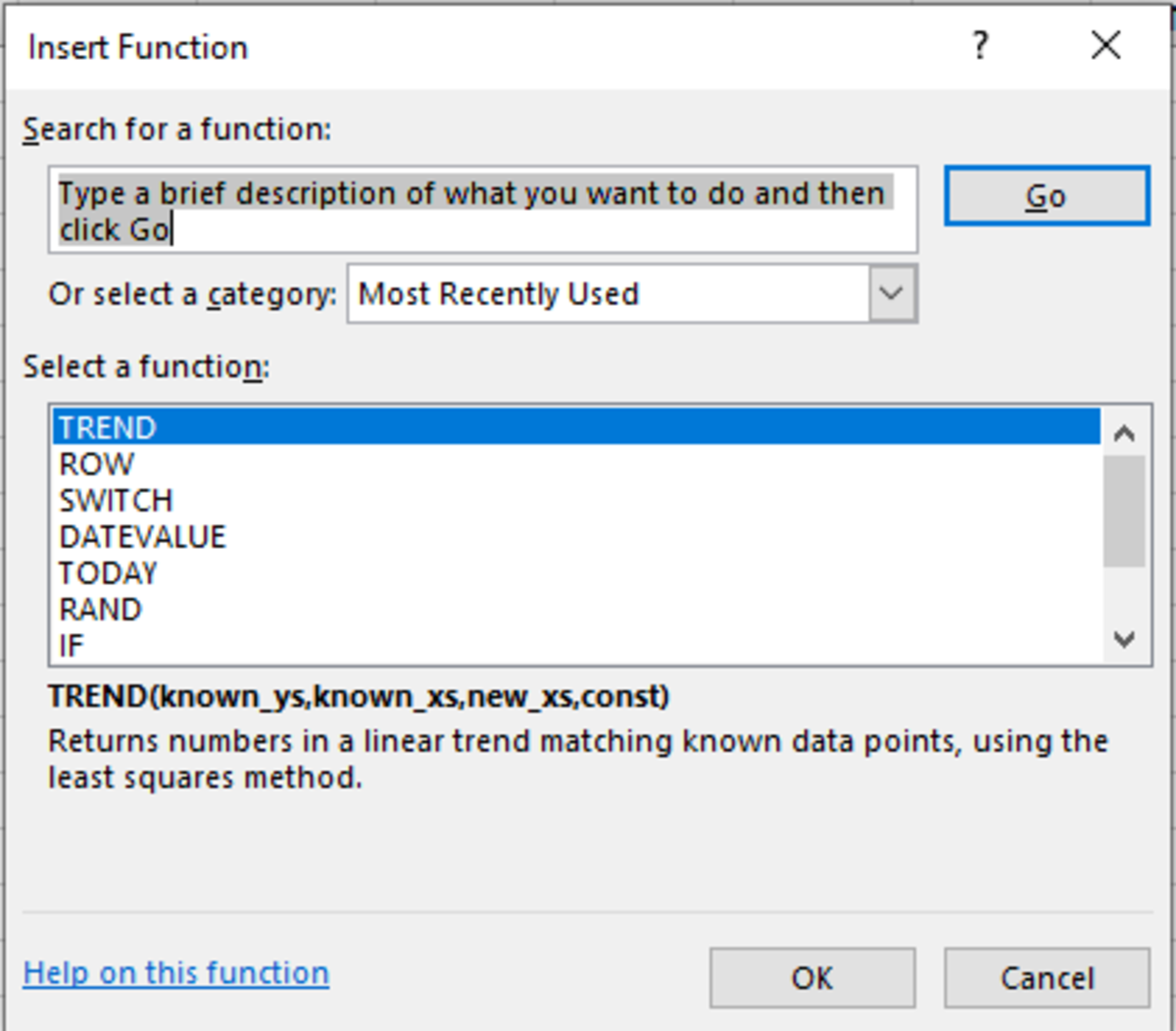
The first thing I’m going to do is select the cell where the first estimated year will show up and then click on the Functions tab in the main tabs section. Next, the Insert function will be selected. The window in the illustration below will appear. Since the function was recently used I can just click on TREND. Otherwise, I would search to find a function that I want to use.
Selecting the Trend Function Using the Insert Method
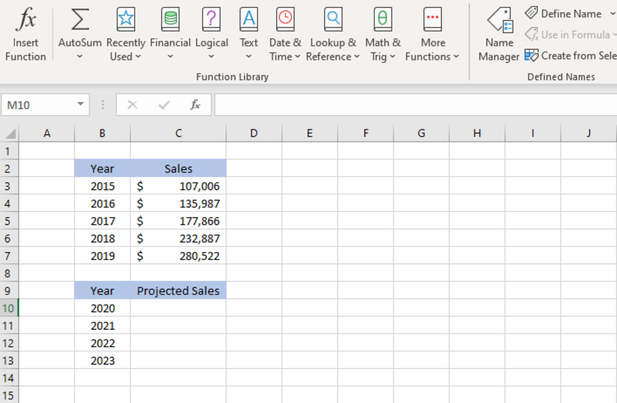
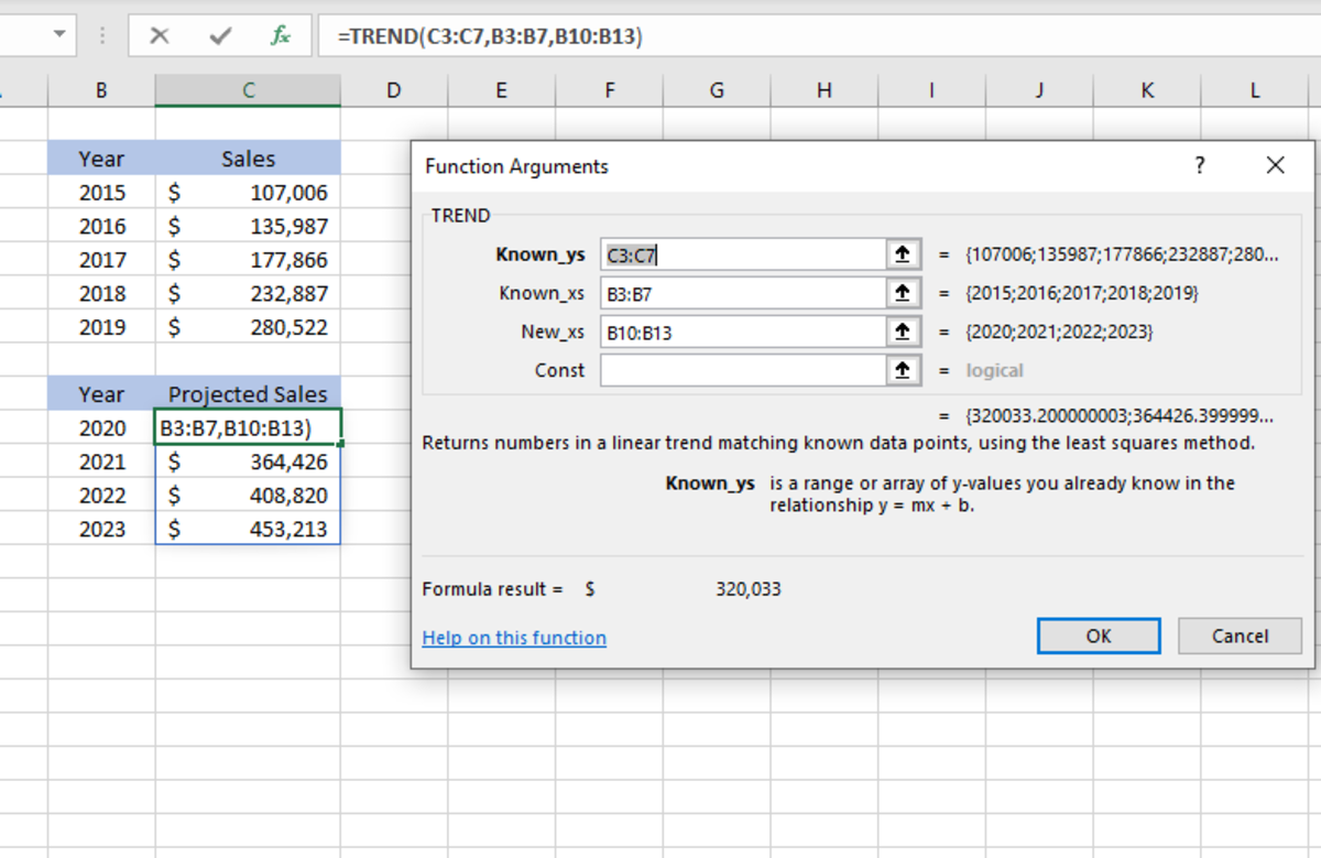
Next, I get to insert all of my ranges. The first would be the array known y values. These are the sales figures that are already known. So, I can select the arrow on the right side of the known y’s field, then select the array. It is now time to select the known x’s. These are going to be the years corresponding to the sales figures that were just selected. Lastly, the unknown x’s are selected. The unknown x’s are the years that I want to return projected y values for. After clicking on the OK button, each of the y values are predicted. Remember that only one cell needs to be used to input the function and the rest of the values will fall into place depending on how many unknown x values are selected.
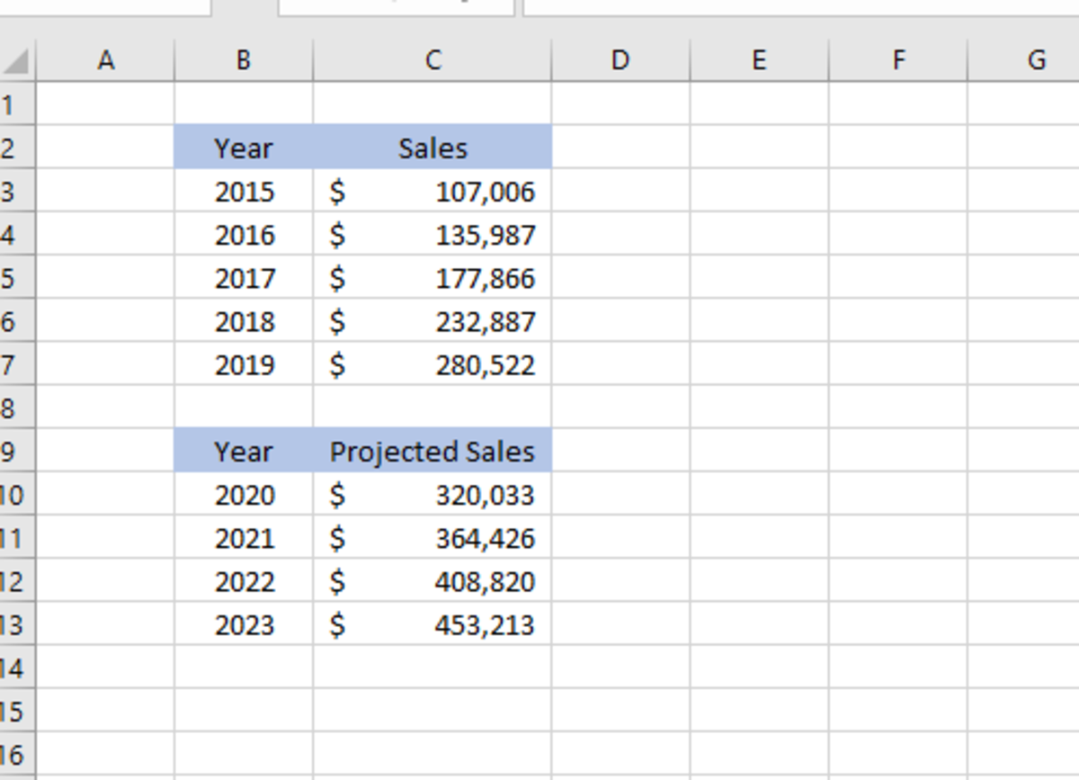
Trend Function Results
Spill Error in Excel
In the event that you get a spill error as a result, make sure that is no data in the cells where the new y values are supposed to appear. For example, if you are looking for the trends for 2021 to 2025, the formula will be placed where the new y value for 2021 will appear while the other years need to remain blank. If you still get errors, I would clear those cells or even try to put your data in a few more times. This content is accurate and true to the best of the author’s knowledge and is not meant to substitute for formal and individualized advice from a qualified professional. © 2020 Joshua Crowder