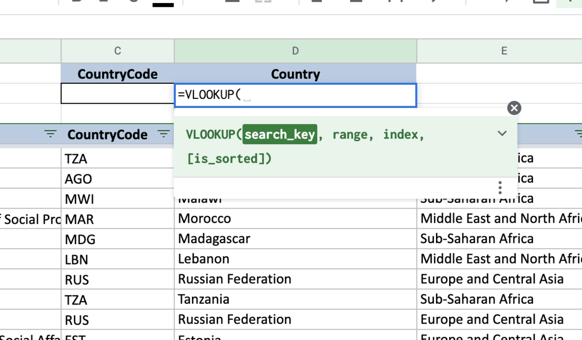
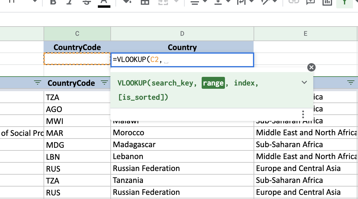
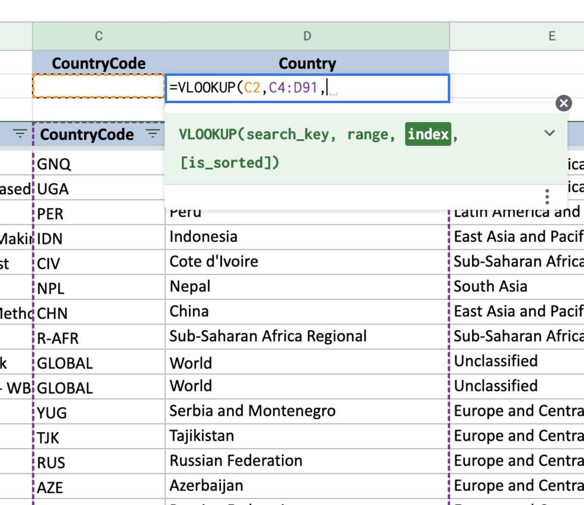
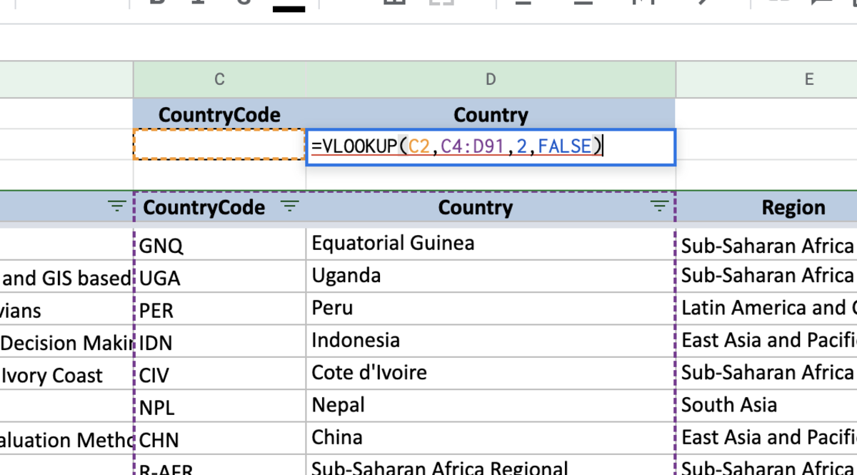
=VLOOKUP(search_key, range, index, [is_sorted])
Value Lookup Example
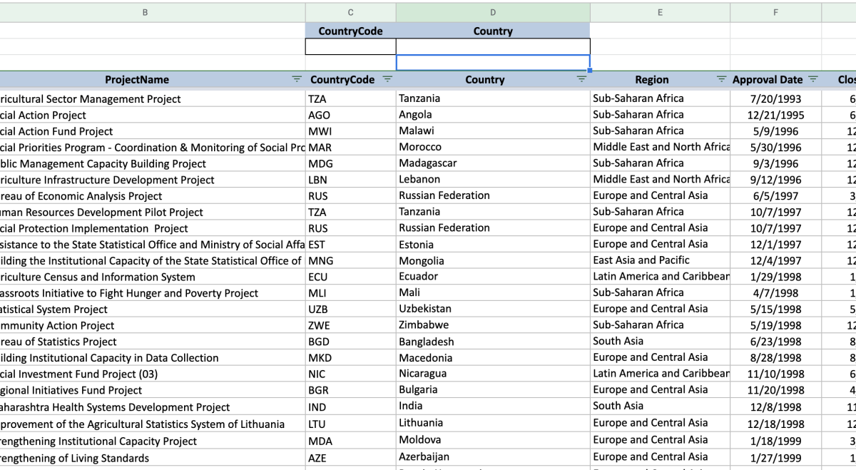
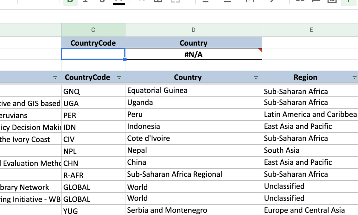
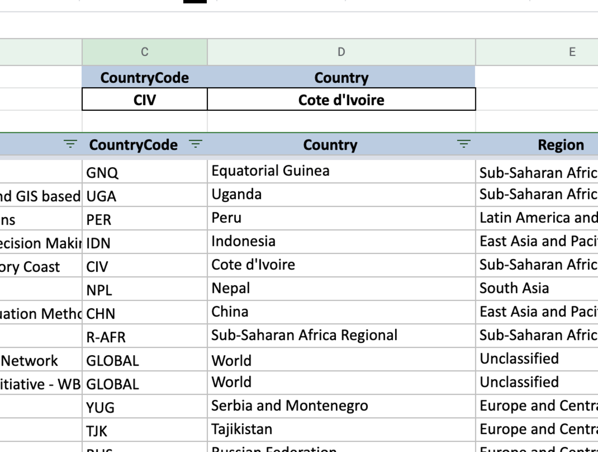
In the example below, we’ll see how to VLOOKUP works with simplicity. I set up an input for the country code and I want the VLOOKUP formula to return the country name with that given country code. The search key will be the value that is being looked up. This will be cell C2 where the lookup or key value will be entered. Next, the range needs to be selected. The range will contain all possible lookup values and the values that will be returned by the function. The next piece of information needed is the index. Since there are only two columns in this range the index will be number 2 since that is where the country name is the value that I want to be returned. When indexing the formula only considers the columns in the range and counts columns from left to right. The last piece of information needed is the sorted section. Since we want to match the country code exactly I want to use an exact match. At first, I received an error because there is now country to look up yet. After adding a country code the VLOOKUP formula is working because the related county was returned in the cell where the formula was inputted. This content is accurate and true to the best of the author’s knowledge and is not meant to substitute for formal and individualized advice from a qualified professional. © 2022 Joshua Crowder