The VLOOKUP Function Syntax
The VLOOKUP function needs to be inputted like a formula for it to be able to work. To add a VLOOKUP formula to a cell, a cell needs to be clicked, and “=VLOOKUP(” needs to be typed in. After the open parenthesis, this is a specific syntax that needs to be followed. VLOOKUP (lookup_value, table_array, col_index_num, [range_lookup]) If the syntax is not followed an error may occur in the field where the formula was written. Each variable needed for the VLOOKUP function is described below. The Vlookup Value This indicates what record to abstract information from. The VLOOKUP function will always search the first column of a table for this value. The record that is chosen will contain data to be returned to the cell that the formula is typed in. The Table Array This lets the function know where all the data is. The whole table being used should be selected so that each record can be indexed. The VLOOKUP value will always be in the first column of the table so you may want to start this selection in column two if that is where the lookup value can be found. The Column Index Number This represents the column that the data to be returned is in. So, the lookup value determines the row and the column index determines the column. What is found when these meet will determine what data will appear in the cell. The Range LOOKUP This is the sensitivity measure and specifies whether the match needs to be approximate or exact. This range is optional and can be left out. Approximate and exact match settings are discussed in more detail below.
Approximate match - To return an approximate match the last input in the formula would need to be TRUE or 1. When this option is chosen the VLOOKUP function will assume that the first column (where the lookup value appears) is sorted alphabetically or numerically and will search for the closest approximate answer. Exact match - To return the exact match the last input in the formula will need to be False or 0. This will ensure that the value being looked up will have to make an exact match.
VLOOKUP Syntax Examples
=VLOOKUP(“Amber”,A1:B100,2,FALSE) In this example, amber will be looked for in the first column of a table. The section of the table used for the lookup is A1 to B100. The data that needs to be returned is in column two of the table. An exact match must be made. =VLOOKUP(A2,A10:C20,2,TRUE) In this example, whatever value is entered into cell A1 will become the lookup value. The section of the table used for the lookup is A10 to C20. The data that needs to be returned is in column two of the table. An approximate match must be made. =VLOOKUP(A2,’Clients’!A:F,3) In this example, whatever value is entered into cell A2 will become the lookup value. The section of the table used for the lookup is located in columns A to F in the client’s worksheet. The data that needs to be returned is in column three of the table.
Inserting a VLOOKUP Function
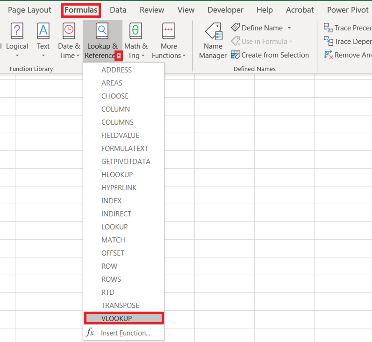
The VLOOKUP function can be inserted into a worksheet cell with the use of an insertion tool. To insert the function one must first select a cell for the formula by clicking on it. Next, the formulas tab needs to be clicked, as well as the “Lookups & References” button on the Excel ribbon. The VLOOKUP option should be selected from the list.
Inserting VLOOKUP Function From Formulas Tab
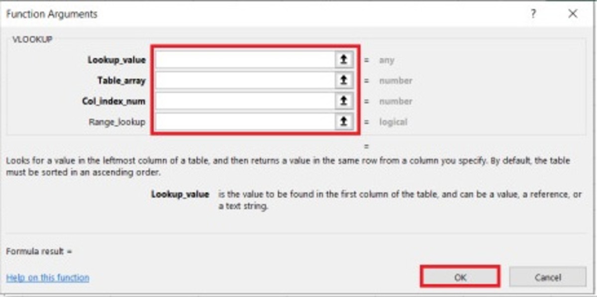
The functions argument window will allow you to add variables to the function. The arrows to the right of each field can be clicked to find cell references or ranges. There are dozens of ways that the VLOOKUP function can be used. Explore the following example if you want to know how this function is typically used in a form.
Example - Using VLOOKUP in a Form
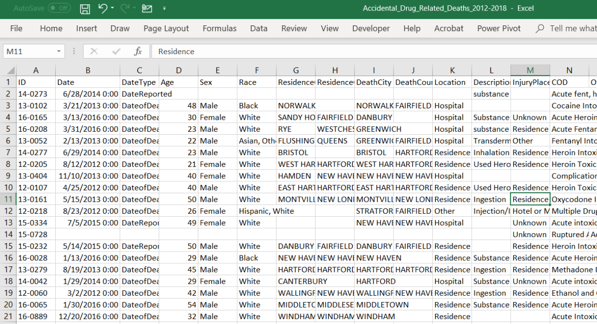
The data in the illustration below shows accidental drug-related deaths from 2012 to 2018. For example, I would like to enter a record ID number in a field and have two pieces of data returned that is an attribute from that record. The mock form that I will create will be in another worksheet in the same workbook. The ID Number will need to be input to return data from the record for sex and cause of death.
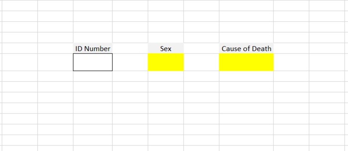
VLOOKUP Form
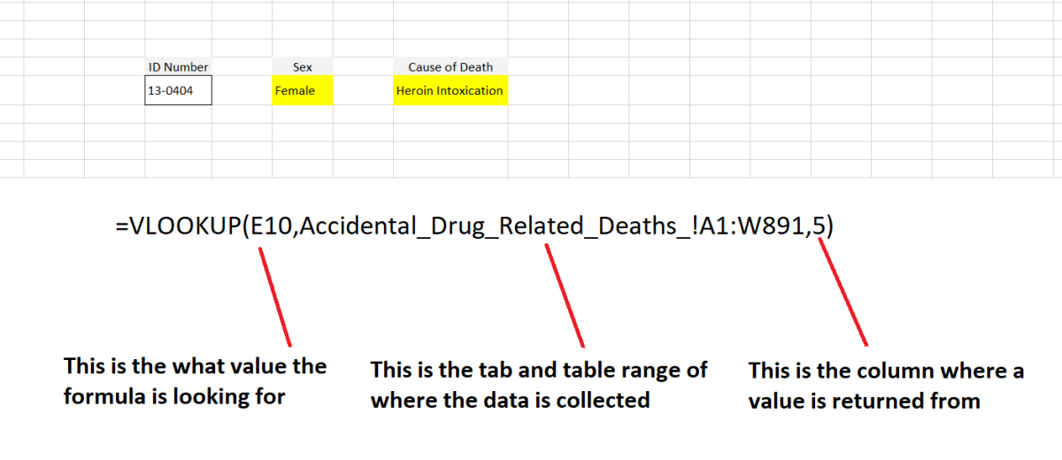
The illustration below shows in detail what was used to determine the value of sex. The lookup value is the value that was entered in E10. That table used for the lookup was located in the range A1 to W891 in the worksheet titled “Accidental_Drug_Related_Deaths_.” Next, by entering 5, the sex of the record was returned for that column. The cause of death data was similarly returned by using column 7 instead of column 5. If you want to return multiple data in different fields you can copy the same formula and change the column number depending on what piece of data you want to appear.
VLOOKUP Function Components
This content is accurate and true to the best of the author’s knowledge and is not meant to substitute for formal and individualized advice from a qualified professional. © 2020 Joshua Crowder