Machine Learning With Causal Inference A Project Summary

Our goal is to combine machine learning with Pearl’s framework to execute a causal inference task.

Tools Used for This Project

Causalnex—Python library that uses Bayesian Networks to combine machine learning and domain expertise for causal reasoning. You can use CausalNex to uncover structural relationships in your data, learn complex distributions, and observe the effect of potential interventions. MLflow—Framework that plays an essential role in any end-to-end machine learning lifecycle. It helps to track your ML experiments, including tracking your models, model parameters, datasets, and hyperparameters and reproducing them when needed. Data Version Control (DVC)—Data and ML experiment management tool that takes advantage of the existing engineering toolset that we are familiar with (Git, CI/CD, etc.).

Data Used

For this project, we are going to use breast cancer diagnosis data from Kaggle (originally from UCI Machine Learning Repository). It contains 33 columns (features) and 569 rows (data). Features are computed from a digitized image of a fine needle aspirate (FNA) of a breast mass. They describe the characteristics of the cell nuclei present in the image. The target variable is called ‘diagnosis’ which holds value M for malignant or B for benign.

Insights Derived From the Data

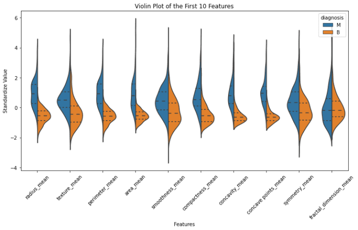
Distribution of Features can be seen using the violet plot; Classification of Features can be seen using the swarm plot and Box plots will help to compare median and detect outliers (all plots show the first 10 features for better visualization).

Causal Graph Implementation and Visualization

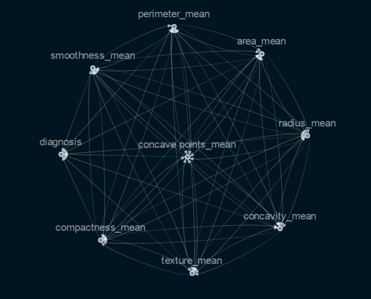
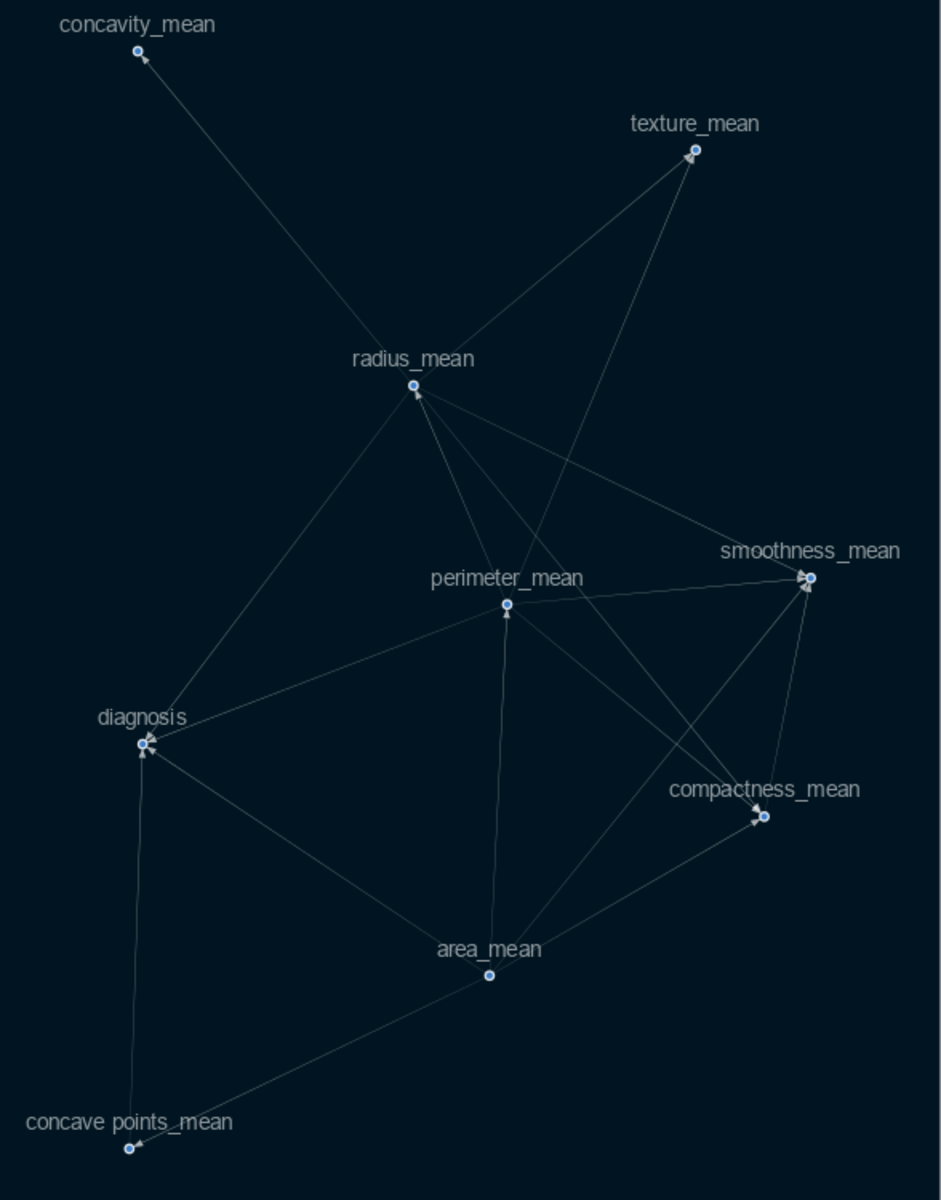
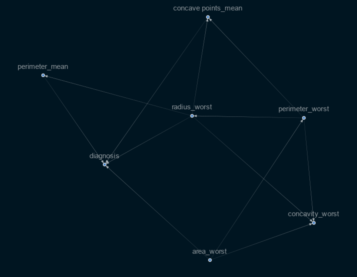
Selecting the variables that are crucial for determining a cause and effect in this situation requires knowledge of or skill in the field of medicine (for our project). Although there are more technical techniques to select the most crucial features, for my project I chose to use important feature metrics discovered using the XgBoost classifier. As a result, I obtained this causal graph. As you can see, the graph is very interconnected and does not clearly show which features directly influence the outcome and which do not. We will therefore employ the Causalnex feature in this case, which thresholds the weaker edges.

Stability of the Graph

The causal graph’s stability will then be tested in the next stage. I, therefore, made several iterations of the above causal graph for this task using subsets of the original data. Then I compared the graphs using the Jaccard Similarity Index, which calculates the intersection and union of the graph edges. The outcomes include:

The similarity between 80% data and 100% data causal graph - 92.6% The similarity between 50% data and 80% data causal graph - 81.43% The similarity between 80% data and 90% data causal graph - 100%

Discretising of the Dataframe Features

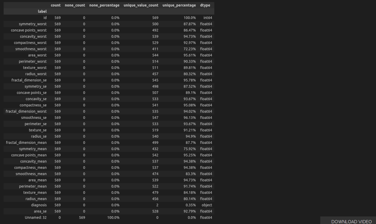
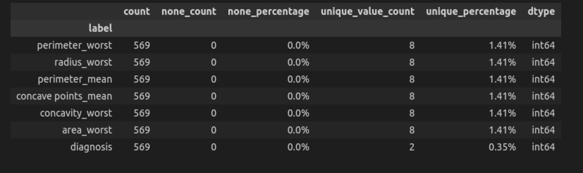
Here we will change the dataframe with continuous data to discrete. We can see below that the values are too unique, which can show that the dataframe consists more of continuous data.

Fitting the Conditional Distribution of the Bayesian Network

It was completed using a discrete version of the original data and the structure model. In order to convert my original data into discrete data, I utilized causalnex’s “DecisionTreeSupervisedDiscretiserMethod.” I was able to predict and obtain scores for the prediction after fitting the Bayesian network.

The accuracy score was 88 % The precision score was 100%

Fitting With Only Directly Connected Graphs

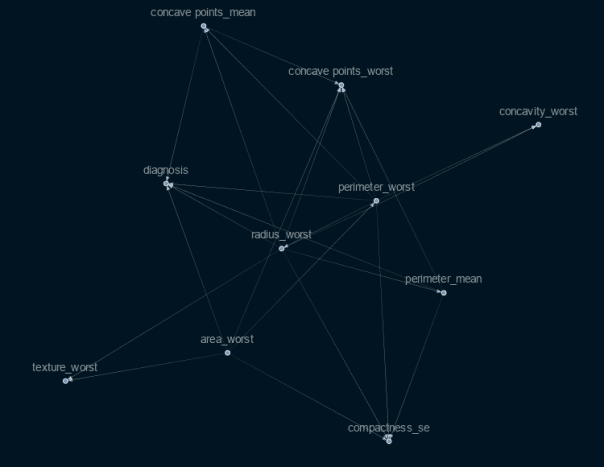
Following the training of this model with all variables, I chose to train a different model with only the factors that directly relate to the target variable (diagnosis), and I obtained the following results:

The accuracy score was 91% The Precision score was 100%

This demonstrates that the graph’s top characteristics can really provide a better prediction than other features that were previously selected. However, although producing good results, the model could not match predictions made using the XgBoost and random forest classifier models.

XgBoost Accuracy score - 97% and Precision score - 97% Random forest Accuracy score - 98% and Precision score - 99%

Conclusion and Future Work

In this project, we examined the use of machine learning and causal inference. We looked at the data, visualized the causal graph, played about with it, and checked to see if it was stable. We were also able to make predictions using the model, which is a good result because making a causal inference is more about determining what caused an event than it is about making predictions. And we saw that we may achieve better results just by utilizing the qualities that were determined through causal inference, which is encouraging for improving implementation and achieving better outcomes. Future work will involve performing various statistics, such as Do-calculus, and finding feature importance using methods so that we can get the most correct graph.