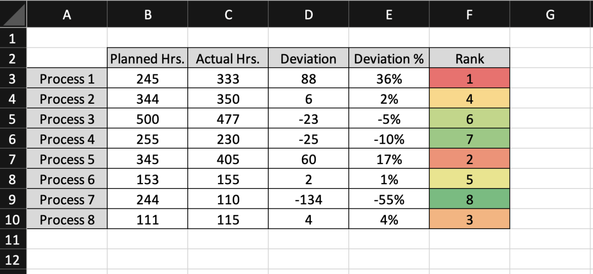
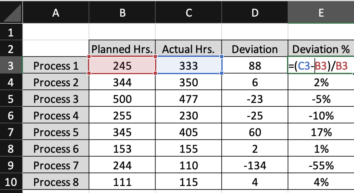
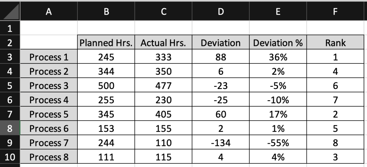
The screenshot below shows planned and actual hour deviations for several processes. Each process has a deviation, deviation percentage, and ranking. Below I walk through the calculations for the deviations followed by how to rank each process by deviation. Steps to rank PVA deviation in this tutorial can be seen below. Step 1. Display Deviation Step 2. Display Deviation % Step 3. Insert the Rank Function Step 4. Add a Color Scale
Step 1. Display Deviation
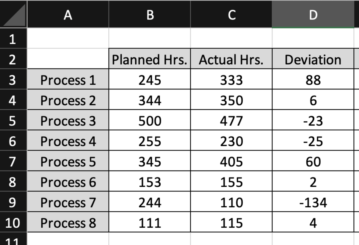
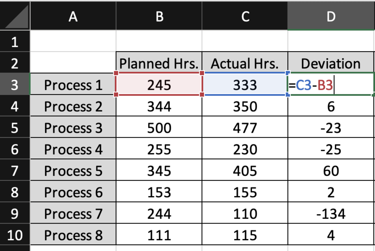
The deviation is the simplest calculation showing the difference between the actual and planned hours where positive numbers show an increase and negative numbers represent a decrease. In this calculation, the planned hours will be considered a fixed base value. The planned hours are subtracted from the actual hours.
Step 2. Display Deviation %
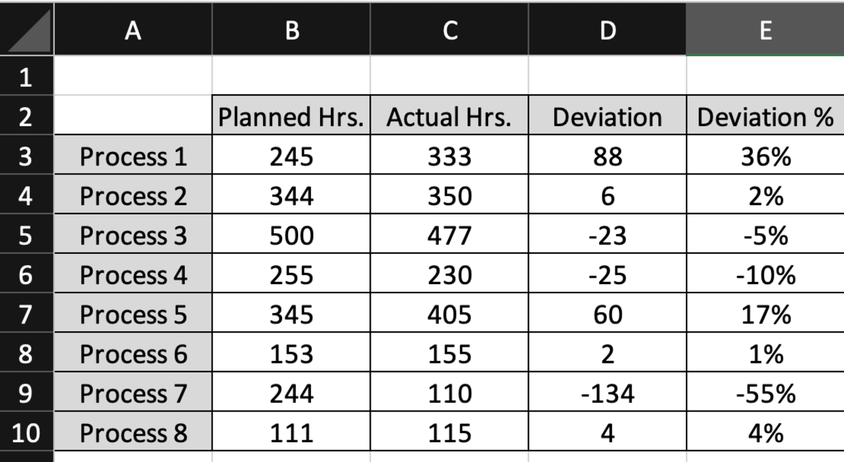
Next, the deviation percentage is calculated in the column labeled Deviation %. The percentage deviation calculation is shown below where the difference between the actual hours and planned hours is divided by planned hours (base value). Some may prefer to use the calculation 1-(B3/C3). I prefer to show the incremental proportion with the historical planned value as a base.
Step 3. Insert the Rank Function
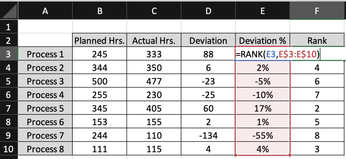
In the last column, each process is ranked. Since there are 8 processes being ranked, all of the processes will be ranked 1-8. The ranking is made possible using the RANK function. To use the RANK function, start by typing the function in the first cell to be ranked. =RANK( Next, add the cell that contains the PVA deviation that needs to be ranked. =RANK(E3, The final argument added to the formula is the whole range of deviations. =RANK(E3,E3:E10) Note that dollar signs will need to be added to the row number to be able to drag the formula to other rows. =RANK(E3,E$3:E$10)
Step 4. Add a Color Scale
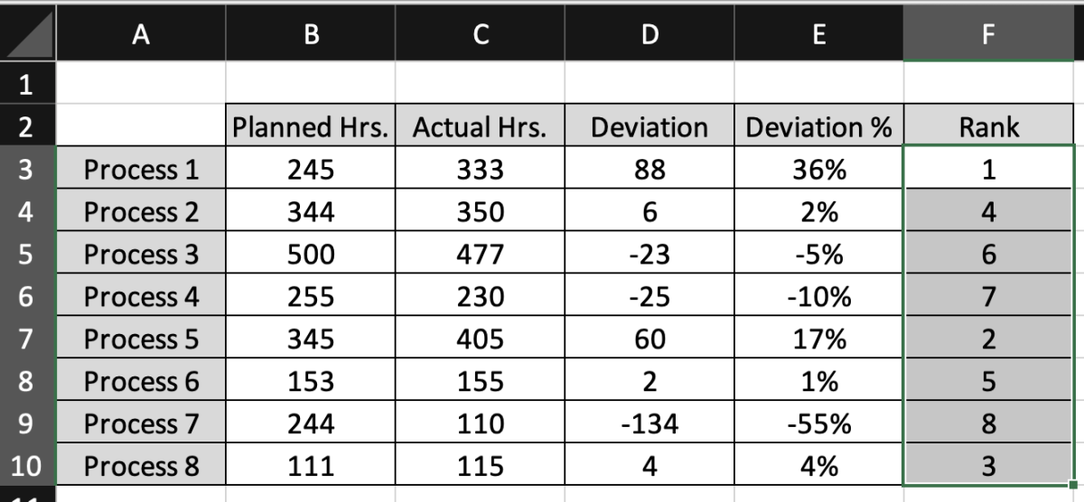
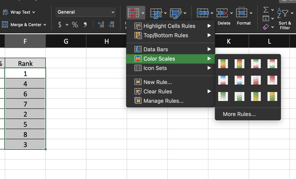
If you would like to add formatting to the ranking column, color scales can be added. Start this process by selecting the column then click on the conditional formatting under the home tab. Select the color scales button and your preferred color scaling option. The color scale option used in the example shows the rank with the highest positive deviation in red and the highest negative deviation in green. Neutral color shades are shown for number rankings close to the center. This content is accurate and true to the best of the author’s knowledge and is not meant to substitute for formal and individualized advice from a qualified professional. © 2022 Joshua Crowder

